How well does evolution find solutions? Richard Harris models population change.
Last time we built a library with which we will simulate the process of evolution in the hope that we can use it to gain some insight into if and how evolution works in the real world. All that was left to do was implement a biochem complex enough to act as an analogue of the relationship between the genetic makeup of a real world creature and its physical properties. What I'd really like to use would be a model of engine efficiency and power such as I used to illustrate the Pareto optimal front.
Unfortunately, such models are complicated. Really complicated. We're talking advanced computational fluid dynamics to even work out what happens inside a piston [ Meinkel97 ].
So instead, I'm going use randomly generated functions with several peaks and troughs. Thankfully, it's really easy to construct such functions by adding together a set of randomly weighted constituent functions, known as basis functions. Specifically I'm going to use radial basis functions, so named because they depend only on how far an evaluated point is from a central point.
There are quite a few radial basis functions to choose from. I shall use one we have already come across; the Gaussian function. This is the probability density function of the normal distribution and has the form
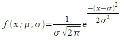
Its shape is illustrated in Figure 1.
|
| Figure 1 |
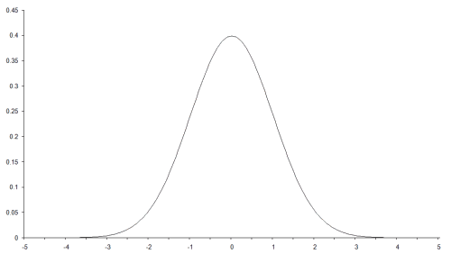
We don't require that the function integrates to one over the entire real line, so shall replace the scaling factor with a simple weighting value. We also want to generalise to more than one dimension so must slightly change the exponentiated term. The functions we shall use will have the form
The || x - μ i || 2 means the square of the straight line, or Euclidean, distance between the points x and and is easily calculated by summing the squares of the differences between each element of the vectors representing the coordinates of those points. Each function in the set will have its own weight w i and they all share a scaling factor c applied to the squared distance. We shall restrict the arguments of our functions to values between zero and one, so I shall choose this scaling factor so that, rather arbitrarily, a distance of 0.1 corresponds to a 50% drop in the value of the function from its maximum at a distance of zero. This implies that
0.5 = e-0.01c
Taking logs of both sides yields
  -0.01c = ln0.5 ≈ -0.7
       c = 70
Figure 2 illustrates one such function, in one dimension, constructed from 8 basis functions with centres randomly chosen from the range 0.2 to 0.8 and weights randomly chosen from the range -1 to 1.
|
| Figure 2 |
Implementing a two dimensional version of this is reasonably straightforward. Listing 1 shows the class definition for our random function.
    namespace evolve
    {
      class random_function :
         public std::binary_function<double,
         double, double>
      {
        class node
        {
        public:
          node();
          double operator()(double x, double y) const;
        private:
          double x_;
          double y_;
          double w_;
        };
        typedef std::vector<node> nodes_type;
      public:
        random_function();
        explicit random_function(size_t nodes);
        double operator()(double x, double y) const;
      private:
        nodes_type nodes_;
      };
    }
|
| Listing 1 |
The node nested class represents a single, randomly centred and weighted, basis function supporting function call semantics through operator() . The random_function class maintains a set of node s and sums the results of the function calls to each of them in its own operator() .
So let's take a look at the implementation of node 's member functions (Listing 2).
    evolve::random_function::node::node() :
       x_(rnd(0.6)+0.2),
       y_(rnd(0.6)+0.2),
       w_(rnd(2.0)-1.0)
    {
    }
    double
    evolve::random_function::node::operator()(
       double x, double y) const
    {
      double d2 = (x-x_)*(x-x_)+(y-y_)*(y-y_);
      return w_*exp(-70.0*d2);
    }
|
| Listing 2 |
I'm a little ashamed to have hard coded the ranges of the central points and weights. However, we're only going to use it during our simulations, so I think it's probably forgivable in this instance.
Now we can take a look at the implementation of random_function . First off, the constructors (Listing 3).
    evolve::random_function::random_function()
    {
    }
    evolve::random_function::random_function(
       size_t nodes)
    {
      nodes_.reserve(nodes);
      while(nodes--) nodes_.push_back(node());
    }
|
| Listing 3 |
Both are pretty simple. The initialising constructor simply pushes the required number of default constructed node s onto the nodes_ collection, relying upon their constructors to randomly initialise them.
The function call operator is also pretty straightforward (Listing 4).
    double
    evolve::random_function::operator()(
       double x, double y) const
    {
      double result = 0.0;
      nodes_type::const_iterator first =
         nodes_.begin();
      nodes_type::const_iterator last  =
           nodes_.end();
      while(first!=last) result += (*first++)(x, y);
      return result;
    }
|
| Listing 4 |
As described before, this simply iterates over the nodes_ , summing the results of each function call.
At long last we're ready to implement a specialisation of biochem (Listing 5).
    class example_biochem : public evolve::biochem
    {
    public:
      explicit example_biochem(size_t nodes);
      virtual size_t genome_base() const;
      virtual size_t genome_size() const;
      virtual size_t phenome_size() const;
      virtual double p_select() const;
      virtual void   develop(
         const genome_type &genome,
         phenome_type &phenome) const;

    private:
      enum {precision=5};

      double make_x(const genome_type &genome) const;
      double make_y(const genome_type &genome) const;
      double make_var(
         genome_type::const_iterator first,
         genome_type::const_iterator last) const;
      evolve::random_function f1_;
        evolve::random_function f2_;
      };
|
| Listing 5 |
The example_biochem treats the genome as a discrete representation of two variables each with precision , or five, digits each. The two random_functions map these variables onto a two dimensional phenome. We hard code the biochem properties to reflect this, as illustrated in Listing 6.
      size_t
      example_biochem::genome_base() const
      {
        return 10;
      }
      size_t
      example_biochem::genome_size() const
      {
        return 2*precision;
      }
      size_t
      example_biochem::phenome_size() const
      {
        return 2;
      }
      double
      example_biochem::p_select() const
      {
        return 0.9;
      }
|
| Listing 6 |
Note that we're sticking with the selection probability of 0.9 that we used in our original model.
The constructor simply initialises the two random_function s with the required number of nodes.
      example_biochem::example_biochem(
         size_t nodes) : f1_(nodes), f2_(nodes)
      {
      }
As you no doubt recall, the develop member function is responsible for mapping from the genome to the phenome and our example does so using the make_x and make_y member functions to create the two variables we need for the random_function s from the genome. (See Listing 7.)
      void
      example_biochem::develop(
         const genome_type &genome,
         phenome_type &phenome) const
      {
        if(genome.size()!=genome_size())
           throw std::logic_error("");
        phenome.resize(phenome_size());
        double x = make_x(genome);
        double y = make_y(genome);
        phenome[0] = f1_(x, y);
        phenome[1] = f2_(x, y);
      }
|
| Listing 7 |
The make_x and make_y member functions themselves simply forward to the make_var member function with each of the two precision digit halves of the genome (Listing 8).
      double
      example_biochem::make_x(
         const genome_type &genome) const
      {
        if(genome.size()!=genome_size())
           throw std::invalid_argument("");
        return make_var(genome.begin(),
           genome.begin()+precision);
      }
      double
      example_biochem::make_y(
         const genome_type &genome) const
      {
        if(genome.size()!=genome_size())
           throw std::invalid_argument("");
        return make_var(genome.begin()+precision,
           genome.end());
      }
|
| Listing 8 |
The make_var function maps an iterator range to a variable between zero and one. It does this by treating the elements in the range as progressively smaller digits, dividing the multiplying factor by the genome_base at each step to accomplish this.
      double
      example_biochem::make_var(
         genome_type::const_iterator first,
         genome_type::const_iterator last) const
      {
        double var = 0.0;
        double mult = 1.0;
        while(first!=last)
        {
          mult /= double(genome_base());
          var += *first++ * mult;
        }
        return var;
      }
|
| Listing 9 |
Since we're using base 10, this is equivalent to simply putting a decimal point at the start of the sequence of digits. The elements 1, 2, 3, 4 and 5 would therefore map to 0.12345.
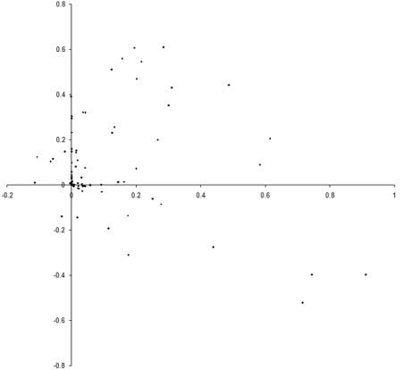
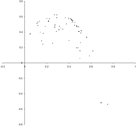
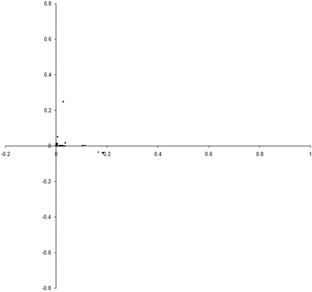
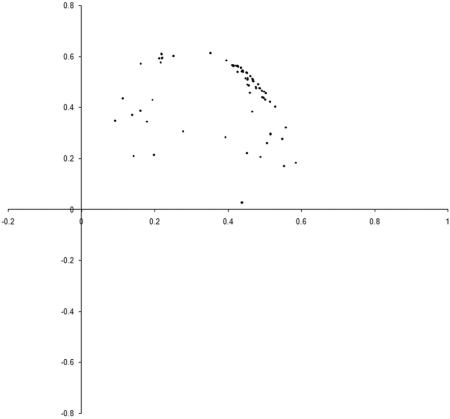
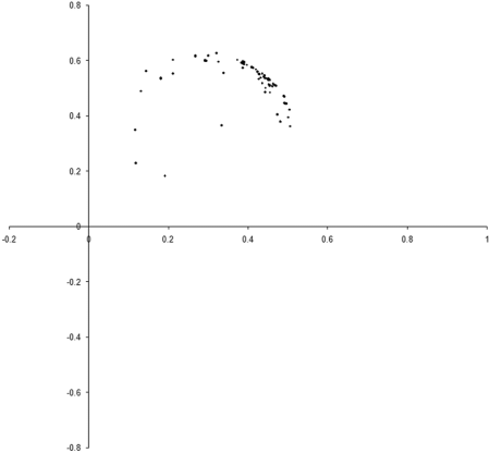
So what are the results of a simulation based on our example_biochem ? Figure 3 illustrates the distribution of the phenomes of a population of 100 individual s from their initial state to their states after 10, 50 and 250 generations.
|
| Figure 3 |
Well, it certainly looks like the population converges to a Pareto optimal front. However, we cannot be certain that there are not any better trade offs between the two functions. To check, we'll need to take a comprehensive sample of the two variables and record the optimal front.
We can do this by maintaining a list of undominated points. As we test each new point, we check to see if it is dominated by any in the list. If not, we remove any points in the list that it dominates and finally add it to the list.
In order to calculate the function values for any point, we first need to add another member function to example_biochem . The function call operator seems a reasonable choice and its implementation is illustrated in Listing 10.
    class example_biochem : public evolve::biochem
    {
    public:
      ...
      std::pair<double, double> operator()(double x,
         double y) const;
      ...
    };
    std::pair<double, double>
    example_biochem::operator()(double x,
       double y) const
    {
      return std::make_pair(f1_(x, y), f2_(x, y));
    }
|
| Listing 10 |
Now we can implement a function to sample the optimal front.
      typedef std::pair<double, double> point;
      typedef std::vector<std::pair<point,
         point> > front;
      front sample_front(size_t n,
         const example_biochem &b);
Note that the std::pair of point s represents the two input variables with its first member and the two elements of the output phenome with its second member.
The implementation of sample_front (Listing 11) follows the scheme outlined above, slicing each of the variables into n samples and iterating over them, filling up the sample of the optimal front.
    front
    sample_front(size_t n, const example_biochem &b)
    {
      front sample;
      for(size_t i=0;i!=n;++i)
      {
        for(size_t j=0;j!=n;++j)
        {
          double x = double(i) / double(n);
          double y = double(j) / double(n);
          point val = b(x, y);
          if(on_sample_front(val, sample))
         {
            remove_dominated(val, sample);
            sample.push_back(std::make_pair(
               point(x, y), val));
          }
        }
      }
      return sample;
    }
|
| Listing 11 |
The two helper functions, on_sample_fron t and remove_dominated , implement the check that a point is not dominated by any already in the list and the removal of any that it dominates respectively. (See Listing 12.)
    bool
    on_sample_front(const point &value,
       const front &sample)
    {
      front::const_iterator first = sample.begin();
      front::const_iterator last  = sample.end();
      while(first!=last &&
               (value.first>=first->second.first ||
                value.second>=first->second.second))
      {
        ++first;
      }
      return first==last;
    }
    void
    remove_dominated(const point &value,
       front &sample)
    {
      front::iterator first = sample.begin();
      while(first!=sample.end())
      {
        if(value.first>=first->second.first &&
           value.second>=first->second.second)
        {
          first = sample.erase(first);
        }
        else
        {
          ++first;
        }
      }
    }
|
| Listing 12 |
Note that the loop condition in on_sample_front and the comparison at the heart of remove_dominated are simply hard coded versions of the complement of the pareto_compare function we developed earlier.
Note that for n samples of each variable, the sample_front function must iterate over n 2 points, making approximately O( n ) comparisons at each step (since the optimal front is a line in the plane). We can't therefore afford to work to the same precision as we do in the simulation itself.
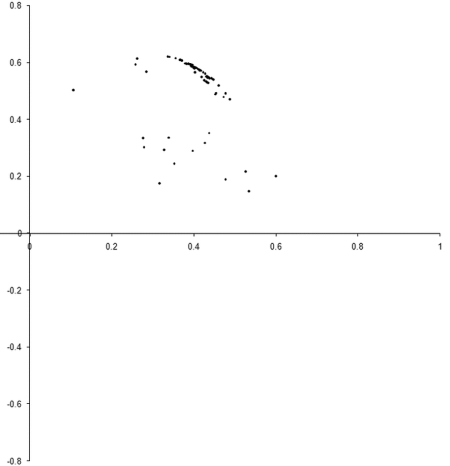
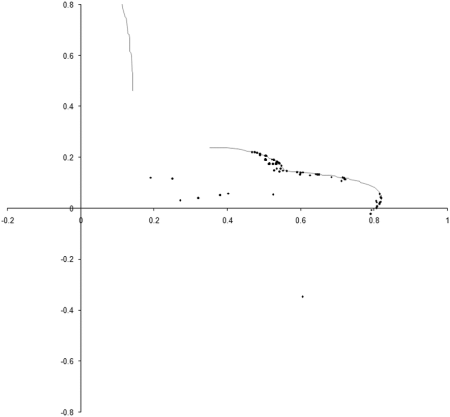
Figure 4 adds the 100 by 100 point sample of the optimal front to the final state of our earlier simulation.
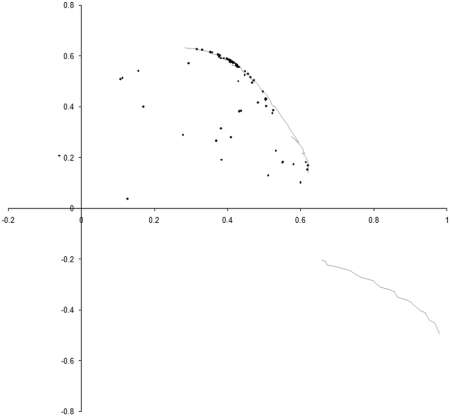
|
| Figure 4 |
Well, our simulation has certainly ended up distributed along part of the optimal front, but seems to have missed an entire section of it. To see why, we need to take a look at how the points whose values lie on the optimal front are distributed.
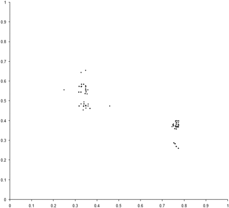
This requires a further change to the example_biochem . To compute the distribution of the variables represented by the genomes, we need to make the make_x and make_y member functions public. Figure 5 compares the final distribution of points in our simulation to the set comprising the sample of the Pareto optimal front.
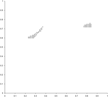
|
| Figure 5 |
Clearly our population has converged on only one of the two regions from which the optimal front is formed. The question is, why?
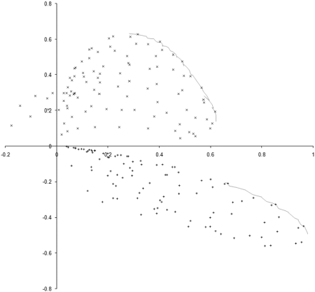
To investigate this, we need to examine the properties of our example_biochem near each of the two regions of the optimal front. We do this by sampling squares of side 0.3 centred on the mid points of the two regions, as illustrated along with the results in Figure 6.
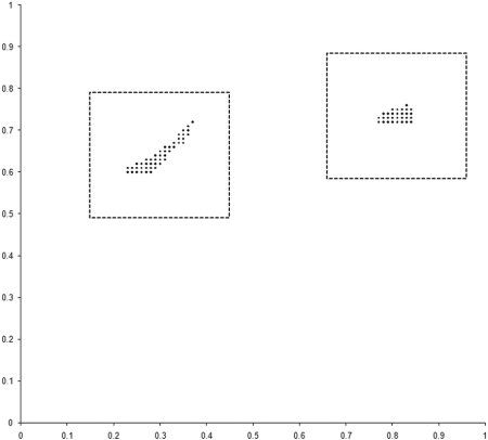
|
| Figure 6 |
The 100 point uniform sample of the two regions clearly shows that points in the region of the rightmost front, marked with + symbols, are dominated by points in the region of the leftmost, marked with x symbols. The evolution process during our simulation has therefore converged on the portion of the optimal front located in the generally better region.
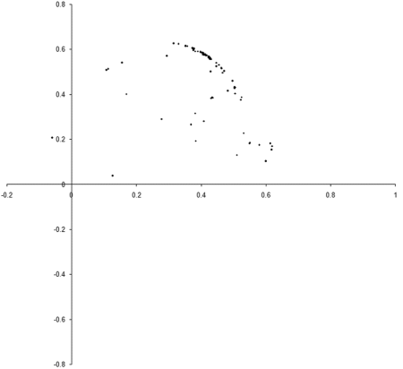
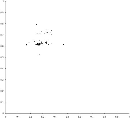
So presumably, if our example_biochem were to have several mutually dominant regions, we should expect to find individuals populating many of them. Well, sometimes, as Figure 7 illustrates.
|
| Figure 7 |
In this case the front is formed from 3 separate regions, of which 2 are represented in the final population . Such regions will not necessarily persist for the duration of a simulation, however. In many cases multiple optimal regions will be populated part way through a simulation, only to disappear by the end. This is due to an effect known as genetic drift, which is also observed in the natural world [ Frankham02 ].
In a small population, a less densely occupied region has a relatively large risk of being out competed by a more densely occupied region. The latter will likely have a greater number of dominant individual s and hence a better chance of representation after selection. The cumulative effect is that the population can converge on a single region, even if that region is not quantitatively better than the other. This can be mitigated with geographically separated sub population s or, in the terms of our model, several independent simulations. If the loss of diversity is solely due to genetic drift, different simulations will converge on different optimal regions and the combination of the final states will yield a more complete picture of the optimal front.
Returning to the argument that evolution cannot create information, only destroy it, one could argue that the success of our simulation is due to the initial random distribution of individual s in the population . Could evolution simply be concentrating on the best region of the initial sample, rather than seeking out novelty?
This question is easily answered by forcing the individual s in the initial population to start at the same point. This requires a couple of minor changes to the individual and population classes.
Listing 13 shows the new constructors we need to add to these classes.
    namespace evolve
    {
      class individual
      {
      public:
        ...
        individual(unsigned long init_val,
           const biochem &b);
        ...
      };
      class population
      {
      public:
        ...
        population(size_t n, unsigned long init_val,
           const biochem &b);
        ...
      };
    }
|
| Listing 13 |
Their implementation is pretty straightforward, replacing the random initialisation of the phenome with assignment to the initial value. (See Listing 14.)
    evolve::individual::individual(
       unsigned long init_val,
       const biochem &biochem) :
       biochem_(&biochem),
       genome_(biochem.genome_size(), init_val)
    {
      develop();
    }
    evolve::population::population(size_t n,
       unsigned long init_val,
       const biochem &biochem) : biochem_(biochem),
       population_(n, individual(init_val, biochem)),
       offspring_(2*n)
    {
    }
|
| Listing 14 |
Note that we don't call reset in the new population constructor since this time we want all of the individual s to be the same.
Figure 8 shows the results of repeating our original simulation with an initial population formed entirely from individual s with zero initialised genomes.
|
| Figure 8 |
Clearly, the initial distribution seems to have had little impact on the final state of the population .
So, given that our simulation has converged on the optimal set of trade offs, or at least the most stable of them, despite starting far from that set, where does the information actually come from?
Well, one further criticism that has been made is that these kinds of simulations somehow inadvertently encode the answers into the process; that we have unconsciously cheated and hidden the solution in the code.
You may be surprised, but I am willing to concede this point. The information describing the best individual s is hidden in the code. Specifically, it's in example_biochem . Whilst we may find it difficult to spot which genomes are optimal simply by examining the complex trade offs between the two functions, it does not mean that the information is not there. The Pareto optimal front exists, whether or not it's easy for us to identify.
However, I do not agree that this represents a weakness in our model.
Just as the information describing the Pareto optimal front is written into our example_biochem , so the information describing the rich tapestry of life we find around us is written into the laws of nature; into physics and chemistry. We simply do not have the wherewithal to read it.
Evolution, however, suffers no such illiteracy. It may not create information, but it is supremely effective at distilling it from the environment in which it operates.
The extraordinary power of evolution has not escaped the computer science community. From its beginnings in the 1960s and 1970s [ Rechenberg65 ] [ Klockgether70 ] [ Holland75 ] the field of evolutionary computing has blossomed [ Goldberg89 ] [ Koza92 ] [ Vose99 ]. Whilst the details generally differ from those of our simulation, the general principles are the same. The quality of a genome is measured by a function, or functions, that model a design problem, say improving the efficiency and reducing the emissions of a diesel engine [ Hiroyasu02 ]. Through reproduction and selection, evolution has repeatedly proven capable of extracting optimal, or at least near optimal, solutions to problems that have previously evaded us [ Hiroyasu02 ].
There are still some aspects of our model that could use some improvement, however. For example, we are not modelling the effect of limited resources during the development of an individual . If you have the time and the inclination, you might consider adapting the code to reflect this, perhaps by introducing some penalty to individual s in densely populated regions.
If you make any further discoveries, I'd be delighted to hear about them.
Acknowledgements
With thanks to Keith Garbutt and Lee Jackson for proof reading this article.
References & Further Reading
[ Frankham02] Frankham, R., Ballou, J. and Briscoe, D., Introduction to Conservation Genetics , Cambridge University Press, 2002.
[ Goldberg89] Goldberg, D., Genetic Algorithms in Search, Optimization, and Machine Learning , Addison-Wesley, 1989.
[ Hiroyasu02] Hiroyasu, T. et al., Multi-Objective Optimization of Diesel Engine Emissions and Fuel Economy using Genetic Algorithms and Phenomenological Model , Society of Automotive Engineers, 2002.
[ Holland75] Holland, J., Adaptation in Natural and Artificial Systems , University of Michigan Press, 1975.
Karr, C. and Freeman, L. (Eds.), Industrial Applications of Genetic Algorithms , CRC, 1998.
[ Klockgether70] Klockgether, J. and Schwefel, H., 'Two-Phase Nozzle and Hollow Core Jet Experiments', Proceedings of the 11th Symposium on Engineering Aspects of Magnetohydrodynamics , Californian Institute of Technology, 1970.
[ Koza92] Koza, J., Genetic Programming: On the Programming of Computers by Means of Natural Selection , MIT Press, 1992.
[ Meinkel97] Meinke1, M., Abdelfattah1, A. and Krause1, E., 'Simulation of piston engine flows in realistic geometries', Proceedings of the Fifteenth International Conference on Numerical Methods in Fluid Dynamics , vol. 490, pp. 195-200, Springer Berlin, 1997.
[ Rechenberg65] Rechenberg, I., Cybernetic Solution Path of an Experimental Problem , Royal Aircraft Establishment, Library Translation 1122, 1965.
[ Vose99] Vose, M., The Simple Genetic Algorithm: Foundations and Theory , MIT Press, 1999.