You're Going To Have To Think!

The dragon of numerical error is not often roused from his slumber, but if incautiously approached he will occasionally inflict catastrophic damage upon the unwary programmer's calculations.

So much so that some programmers, having chanced upon him in the forests of IEEE 754 floating point arithmetic, advise their fellows against travelling in that fair land.

In this series of articles we shall explore the world of numerical computing, contrasting floating point arithmetic with some of the techniques that have been proposed as safer replacements for it. We shall learn that the dragon's territory is far reaching indeed and that in general we must tread carefully if we fear his devastating attention.

On the classification of numbers

As programmers we are probably aware that integers and floating point numbers have different properties, even if we haven't spent a great deal of time thinking about their precise nature.

However, I rather suspect that we are somewhat less aware of how they fit into the general mathematical classification of number types.

Therefore, before we start looking at the various techniques for representing numbers with computers I should like to explore what exactly it is we mean by Number .

The concept of Number has been refined throughout history as generations of mathematicians have time and again stumbled across inconsistencies in their understanding.

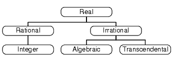
A hierarchy of number types as we currently understand them is provided in figure 1.

Figure 1

Traversing this tree from left to right, we more or less recover the sequence of development in our concept of Number from prehistory to the modern day.

The story of Number begins with the integers, or more accurately the natural numbers; those whole numbers greater than zero. Animal studies have shown that primates, rats and even some birds have a rudimentary ability to count; presumably using neural circuitry similar to that we use to distinguish at a glance between three and four objects, but not between nineteen and twenty. It is not unreasonable, therefore, to suppose that awareness of the natural numbers predates man.

The negative numbers are, comparatively, an example of striking modernity having been discovered in India just a few millennia ago.

The integers, as important as they are, are not particularly useful for measurement; the distance between the ziggurat and the brothel is never quite a whole number of cubits, for example. For this task we instead employed the fractions, or rationals; those numbers equal to the ratio of two integers. Note that the rationals are a superset of the integers; every integer is trivially the ratio of itself and 1.

For many years it was thought that the rationals comprised the totality of Number. Legend has it that a member of the school of Pythagoras discovered that the square root of 2 could not be expressed as a fraction and that his compatriots were so put out by this fact that they drowned him (we shall revisit this in a later article).

The algebraic irrationals are those numbers which are roots of polynomial equations with rational, or equivalently integer, coefficients. By roots we mean those real values, if any, at which the polynomial equates to zero.

The square root of 2 is a root of the polynomial x 2 -2, for example. Technically, the algebraic numbers are a superset of the rationals since the latter are solutions to linear equations with integer coefficients.

The final breed of numbers, the transcendentals, is the most elusive. These are the numbers which are not solutions of polynomial equations with rational coefficients and include such notable numbers as p and e . They are so difficult to identify that it is still not known whether the sum of p and e is itself transcendental. Despite this, it is known that the transcendentals form the vast majority of numbers; if you were to throw a dart at a line representing the numbers between 0 and 1, you would almost certainly hit a transcendental.

To understand why, we need to discuss the mathematics of infinite sets.

Transfinite cardinals

In the late 19 th century Georg Cantor perfected the theory of infinite sets. The transfinite cardinals are not, as their name suggests, characters in a Catholic science fiction blockbuster, but are in fact those infinite numbers that denote the size of infinite sets.

Cantor identified the smallest of the transfinite cardinals, the size of the integers, as . This is known as the countable infinity since we can imagine an algorithm that, given infinite time, would step through them sequentially, counting them off one at a time.

He then asked the question of whether the rationals were larger than the integers; whether they were uncountable. His proof that they were not is one of the most elegant in all of mathematics.

When we say a set is countable, we strictly mean that it can be put into a one to one correspondence with the non-negative integers. For example, the integers are countable since we can map from the non-negative integers to them with the rules

1. if n is even, n maps to ½n
2. if n is odd, n maps to -½(n+1)

Enumerating this sequence yields

0, -1, 1, -2, 2, -3, 3, ...

which clearly counts through the integers, one at a time.

Cantor laid out the rationals such that the numerator (the number on top of the fraction) was indicated by the column and the denominator (the number on the bottom of the fraction) was indicated by the row, as shown in figure 2.

What Cantor realised was that, whilst each row and column stretched on forever and so couldn't be counted one after the other, the diagonals between the first column of a given row and the first row of the corresponding column were all finite and hence countable. For example, we could iterate over the first row, counting diagonally backwards through the table until we hit the first column yielding the sequence

1/1, 2/1, 1/2, 3/1, 2/2, 1/3, 4/1, 3/2, 2/3, 1/4, ...

If we skip any number we have seen before, we have the sequence

1, 2, 1/2, 3, 1/3, 4, 3/2, 2/3, 1/4, ...

So, rather surprisingly, despite there being an infinite number of fractions between any two different integers, the sizes of the set of fractions and the set of integers are in fact equal.

Cantor proceeded to demonstrate that the set of polynomial equations with integer coefficients is also countable and, since each has a finite number of roots, so are the algebraic numbers.

He did this by defining a function, we shall call it c , that takes a polynomial with integer coefficients and returns a positive integer. It operates by adding together the absolute values of the coefficients and the largest power to which the variable is raised, the order of the polynomial, minus one.

For example

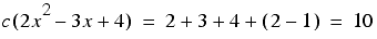
Note that we can insist that the term with the highest order is positive, since multiplying a polynomial by minus one doesn't affect its roots.

Cantor realised that every possible value of this function is shared by a finite number of such polynomials. For example, there are just 4 such polynomials for which this function yields 2.

So we can count off these polynomials by counting through the positive integers and, for each of them in turn, enumerating the members of the finite set of them for which Cantor's function returns that value.

We are left with the question of whether or not the transcendental numbers are of the same size.

If the transcendental numbers are countable then the real numbers, being the union of both they and the algebraic numbers, must be countable too since we could simply alternate between the sequences of each of them.

Cantor noted that if the reals were countable we could construct a list of them as they are generated by the mapping from the integers. Figure 3 illustrates what this list might look like for the numbers between 0 and 1.

Now starting after the decimal point in the first row and moving diagonally down and to the right we can construct a new number

This number is clearly between 0 and 1, but must differ from every number in the list at no less than one digit. Note that we add 2 to each digit rather than 1 to avoid the irritating corner case of recurring nines, such as 0.099999... being equal to 0.1.

We have thus found a number between 0 and 1 that was not in our list and hence the list is incomplete. It is not, therefore, possible to construct such a list and hence the reals, and consequently the transcendentals, are uncountably infinite. Being more sizable than the other numbers, their cardinal number is denoted by .

IEEE 754-1985

So now we know the mathematical classification of numbers we are ready to start looking at how we might implement numeric types with computers.

The IEEE standard [ IEEE ] defines floating point numbers to have a format similar to the scientific notation many of us will recognise from our calculators and spreadsheets. In the familiar decimal base 10 this means a number between 1 and 10 multiplied by 10 raised to the power of another number.

For example, the number of days in a year is approximately 365.

Dividing by this 100 gives us a number between 1 and 10, namely 3.65.

Since 100 is 10 raised to the power of 2, the number of days in the year can be written as 3.65 × 10 2 , or commonly 3.65E2.

The number that we multiply by the power of 10 is known as the mantissa and the power of 10 by which we multiply it is known as the exponent.

Since base 10 is rather inconvenient from a computing perspective, IEEE floating point numbers are defined in the binary base 2. Specifically, numbers are defined as ± b × 2 a with, in the single precision format, the sign taking one bit, the exponent a taking 8 bits and the mantissa b taking 24. Much as in decimal the mantissa must lie between 1 and 10, so in binary it must lie between 1 and 2. The leading digit must therefore be 1, and we can represent b with 23 bits rather than the full 24.

There is, in fact, a special case when we assume the leading digit is 0 rather than 1. This occurs when the exponent takes on its most negative value, yielding the very smallest floating point numbers. Since the leading digits of these numbers, known as subnormal or denormalised numbers, may be 0 there may consequently be fewer bits left to represent the mantissa resulting in fewer significant digits of accuracy, or equivalently in lower precision. In contrast recall that normal numbers have an implied leading digit of 1 and consequently have the full 24 bits with which to represent the mantissa.

In addition to the normal and subnormal numbers, IEEE 754 defines bit patterns to represent the positive and negative infinities and a set of error values for invalid calculations known as the NaNs, for Not a Number. Many of us are probably aware of the quiet and signalling NaNs identified by std::numeric_limits , but perhaps not of the fact that there are actually 2 24 -2 of them in the single precision format, allowing for error codes to be embedded in invalid results.

Figure 4 enumerates the full set of IEEE 754 single precision floating point numbers, ±a 1 a 2 a 3 ...a 8 b 1 b 2 b 3 ...b 23

Note that since the mantissa is finite, floating point numbers are actually a finite subset of the rational numbers and it is vitally important not to confuse them with real numbers.

Double precision

Double precision floating point numbers have precisely the same layout as single precision floating point numbers, differing only in that they have an 11 bit exponent and a 53 bit mantissa. Recall that one of the bits in the mantissa is implied, so that these and the sign bit fill 64 bits.

Henceforth, we shall assume that the double precision format is being used.

Now that we have covered the mundane implementation details of floating point numbers it is time to start looking at the rather more important topic of their precise behaviour.

Not a number

The NaNs infect any calculation they come into contact with since the result of any operation upon a NaN yields a NaN.

Furthermore, any comparison involving a NaN is always false, even an equality comparison between two NaNs.

If you keep this in mind when designing loops and branches, you can ensure that your algorithms will behave predictably in the face of invalid arithmetic operations.

Overflow

Floating point numbers overflow in a satisfyingly predictable way, namely to plus or minus infinity.

Dividing any finite number by an infinity will yield zero and dividing any non-zero number by zero will yield an infinity of the same sign as that number. Adding or subtracting any finite number to or from an infinity will result in that infinity.

These properties mean that many numerical algorithms can implicitly cope with numerical overflow since arithmetic operations and comparisons are internally consistent and, accompanied by some vigorous hand waving, mathematically sound.

Note that dividing 0 by 0, dividing an infinity by an infinity, multiplying an infinity by 0 and subtracting an infinity from itself all yield NaNs.

Rounding error

One of the most common surprises facing the programmer using floating point arithmetic stems from the fact that there are a fixed number of bits with which to represent the mantissa.

We can illustrate the problem by considering decimal notation. Say we restrict ourselves to 4 figures after the decimal point. Assuming that we have chosen the closest number in this representation, x , to a given number we can only say that its true value lies somewhere within x ±5E10 -5 . For example, given π to 4 decimal places, 3.1416, we can only state with certainty that it lies between 3.14155 and 3.14165.

Similarly, for an IEEE double precision floating point number x with an exponent of a , we can only be sure that the true value is between x ±2 a -53 . Conveniently, since normalised floating point numbers have a implicit leading digit of 1, these bounds can be written as x (1±2 -53 ) or, conventionally, as x (1±½ ε ).

Of course, this means that operations on denormalised numbers will introduce proportionally even greater errors but we shall ignore this fact in our analyses and effectively treat them as if they behave in the same fashion as zero.

If an algorithm really must treat denormalised numbers with the same respect as normalised numbers, it will require much more careful analysis.

The mathematical operations of addition, subtraction, multiplication, division, remainder and square root are required by the IEEE standard to be accurate to within rounding error. Specifically, they must return the correctly rounded representation of the result of performing the actual calculation with real numbers. This means that, if using round to nearest, they will introduce a proportional error no larger than (1±½ ε 0).

Note that because of these accumulated rounding errors, equality comparisons between floating point numbers often behave counter-intuitively; values of unlike expressions that should mathematically be equal may have accumulated slightly different rounding errors.

In general, we should prefer to test whether two floating point numbers are similar to each other rather than the same.

Condition number

It is important to note that the rounding guarantees of the IEEE arithmetic operations do not take into account any rounding error in their arguments.

We can capture the sensitivity of the result of a function f to rounding errors in its argument x with the condition number, given by

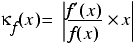
where f' is the derivative of f and the vertical bars mean the absolute value of the expression between them.

This value is approximately equal to the absolute value of the ratio between the relative error of f ( x ) and the relative error of x , as shown in derivation 1. Note that it assumes that f can be calculated exactly and so the condition number does not take into account rounding during the calculation or of the result.

Given a real value x and the nearest normal floating point x* we have The relative error in f is given by 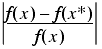Dividing by the relative error in x , we have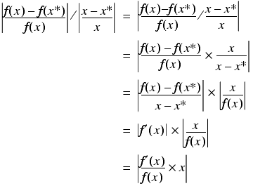

Derivation 1

As an example, consider the exponential function e x whose derivative is equal to e x for all x . Its condition number is therefore | x |, meaning that its relative error at x before rounding is approximately equal to |½ ε x |.

When the condition number is large, a calculation is said to be poorly conditioned and we cannot trust that it is accurate to many digits of precision.

Noting that the number of digits of precision is approximately equal to the logarithm of the reciprocal of the absolute relative error, we can use the condition number to estimate the number of decimal digits of precision of a calculation.

Specifically, we use

where log 10 is the base 10 logarithm, as demonstrated in derivation 2. This is equivalent to subtracting the log of the condition number from the number of digits of precision of the floating point type.

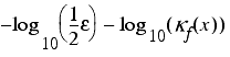
Assuming that the floating point epsilon has n decimal leading zeros, for a given real number and its closest normal floating point number we have where b is between 1 and 10. Now 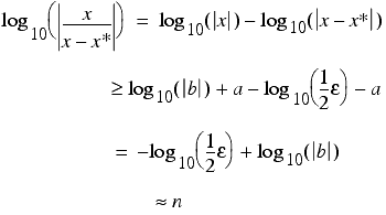Defining the absolute relative error in the result of a function f as 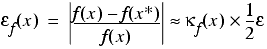we have and hence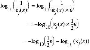

Derivation 2

Cancellation error

Given enough operations or poorly conditioned functions, rounding error can significantly affect the result of a calculation, but it is by no means the worst of our troubles.

Far more worrying is cancellation error which can yield catastrophic loss of precision. When we subtract two almost equal numbers we set the most significant digits to zero, leaving ourselves with just the insignificant, and most erroneous, digits.

For example, suppose that we have two values close to p , 3.1415 and 3.1416. These values are both accurate to 5 significant figures, but their difference is equal to 0.0001, or 1.0E-4, and has just 1 significant figure of accuracy.

Whilst rounding error might sneak up upon us in the end, cancellation error is liable to beat us about the head with a length of two by four.

The poster child of cancellation error is the approximation of numerical differentiation with the forward finite difference. The derivative of a function f at a point x is defined as the limit, if one exists, of

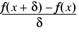
as δ tends to zero.

The forward finite difference replaces the limit with a very small, but non-zero, δ and is a reasonably obvious way to approximate the derivative.

It is equally obvious that we should choose δ to be as small as possible, right?

Wrong!

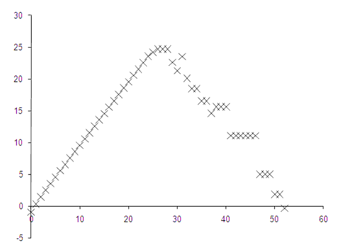
To demonstrate why not, consider the function e x whose derivative at 1 is trivially equal to e . Figure 5 plots a graph of minus the base 2 logarithm of the absolute error in the approximate derivative at 1, roughly equal to the number of correct bits, against minus the base 2 logarithm of δ , equal to the number of leading zeros in its binary representation.

Figure 5

Clearly, decreasing δ works up to a point as indicated by an initial linear relationship between the number of leading zeros and the number of accurate bits. However, this relationship seems to break down beyond δ equal to 2 -25 and the best accuracy occurs when δ is equal to 2 -26 .

From the Taylor series expansion of f we have From this we can obtain the result of the approximate derivative Assuming that we can exactly represent both x and x + δ and that f is accurate to machine precision, the floating point result of this formula will be which is equal to 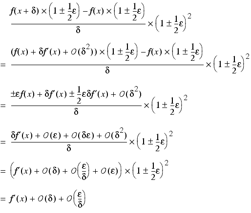Hence, if δ is too large the Ο ( δ ) term will introduce significant errors into the approximation, whereas if it is too small the Ο ( ε / δ ) will do so instead. With some vigorous hand waving, we can ignore the constant factors in these terms, and conclude that since a choice of δ = ε ½ results in them both having the same order of magnitude it is, in some sense, optimal.

Derivation 3

This is suspiciously close to half of the number of bits in the mantissa of a double precision floating point number. In fact it can be proven, under some simplifying assumptions, that the optimal choice for δ is the square root of ε , which has roughly that many leading zeros.

The reason for this behaviour is that, as d gets very small, the results of the two calls to f get very close together and their difference introduces a large cancellation error, as shown formally in derivation 3.

Note that since cancellation error results from the dramatic sensitivity of the subtraction of nearly equal numbers to the rounding errors in those numbers, it can be captured by the condition number.

For example, the expression x -1 has a condition number of | x /( x -1)|. As x tends to 1, the condition number tends to infinity, reflecting the growing effect of cancellation error on the result.

Order of execution

The final surprising aspect of floating point numbers is that the exact order in which operations are performed can have a material effect on the result.

For example, suppose that we wish to calculate the cube of the square root of a number, or equivalently the square root of the cube. Starting out with a value x accurate to within rounding, we have

Next, we take the square root, introducing another rounding error

Finally we multiply it by itself twice to recover the cube, introducing two more rounding errors

Now let's try it in the reverse order. This time we perform the two multiplications first yielding

Secondly we take the square root, introducing one additional rounding error

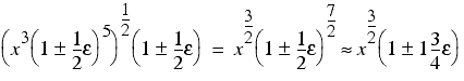
Surprisingly, this second version of the calculation has accumulated just a little more than half the error that the first had.

Whilst this is a relatively simple example, the fundamental lesson is sound; in order to control errors when using floating point numbers we must plan our calculations with care.

You're going to have to think!

I recently read a comment on a prominent IT internet forum proposing that scientists should not be trusted to implement their own computer models since, presumably unlike the comment's author, they are not trained in computer science and are consequently likely to make mistakes. The given example of such a mistake was the calculation of the average of 20 or so values in the low 20s ¹ which was ironic, since a computer scientist should be able to demonstrate that the result of performing this calculation with double precision floating point is correct to about 15 decimal digits of precision!

Such unfair criticism of floating point is not particularly unusual, is often unduly concerned with rounding error and hardly ever mentions the vastly more important topic of cancellation error. One can only assume that many computer science graduates have forgotten their numerical computing lectures and have generalised the very specific and predictable failure modes of floating point arithmetic to the rule of thumb that any use of floating point renders a program broken by design.

These criticisms are generally accompanied by suggestions of alternative arithmetic types that fix the perceived problems with floating point. We shall investigate these in coming articles in this series and we shall learn that if we wish to use computers for arithmetic calculation we shall have to accept the fact that we are going to have to think.

References and further reading

[IEEE] IEEE standard for binary floating point arithmetic. ANSI/IEEE std 754-1985, 1985.

1 Which, given recent events, should be a fairly big hint as to which scientists were being so criticised.