We’ve looked at several approaches to numeric computing. Richard Harris has a final attempt to find an accurate solution.
In this series of articles we have discussed floating point arithmetic, fixed point arithmetic, rational arithmetic and computer algebra and have found that, with the notable exception of the unfortunately impossible to achieve infinite precision that the last of these seems to promise, they all suffer from the problems that floating point arithmetic is so often criticised for.
No matter what number representation we use, we shall in general have to think carefully about how we use them.
We must design our algorithms so that we keep approximation errors in check, only allowing them to grow as quickly as is absolutely unavoidable.
We must ensure that these algorithms can, as far as is possible, identify their own modes of failure and issue errors if and when they arise.
Finally, we must use them cautiously and with full awareness of their numerical properties.
Now, all of this sounds like hard work, so it would be nice if we could get the computer to do the analysis for us.
Whilst it would be extremely difficult to automate the design of stable numerical algorithms, there is a numeric type that can keep track of the errors as they accumulate.
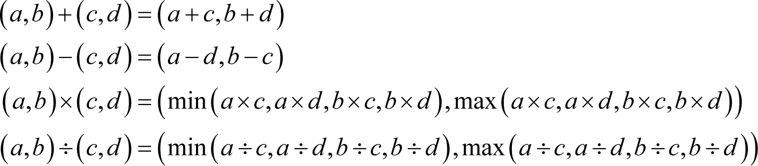
Interval arithmetic
Recall that, assuming we are rounding to nearest, the basic floating point arithmetic operations are guaranteed to introduce a proportional error of no greater than 1±½ε.
It's not wholly unreasonable to assume that more complex floating point functions built into our chips and libraries will also do no worse than 1±½ε.
This suggests that it might be possible to represent a number with upper and lower bounds of accuracy and propagate the growth of these bounds through arithmetic operations.
To capture the upper and lower bound of the result of a calculation accurately we need to perform it twice; once rounding towards minus infinity and once rounding towards plus infinity.
Unfortunately, the C++ standard provides no facility for manipulating the rounding mode.
We shall, instead, propagate proportional errors at a rate of 1±1½ε since we shall be able to do this without switching the IEEE rounding mode. Specifically, we can multiply a floating point result by 1+ε to get an upper bound and multiply it by 1-ε to get a lower bound. The rate of error propagation results from widening the 1±½ε proportional error in the result by this further 1±ε to yield the bounds.
Naturally, this will not work correctly for denormalised numbers since they have a 0 rather than a 1 before the decimal point, so we shall have to treat them as a special case. Specifically, rather than multiplying by 1±ε, we shall add and subtract the smallest normal floating point number, which is provided by std::numeric_limits<double>::min(), multiplied by ε.
Before we apply rounding error to the upper and lower bounds of the result a calculation we shall want them to represent the largest and the smallest possible result respectively. We therefore define the basic arithmetic operations as follows.
As an example, consider the square root of 2. Working with 3 accurate decimal digits of precision, this would be represented by the interval
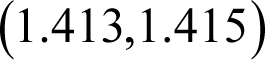
Squaring this result would yield

or
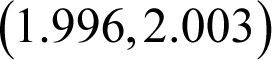
which clearly straddles the exact result of 2 and furthermore gives a good indication of the numerical error.
Unfortunately, as is often the case, the devil is in the details.
The first thing we need to decide is whether the bounds are open or closed; whether the value represented is strictly between the bounds or can be equal to them. If we choose the former we cannot represent those numbers which are exact in floating point, like zero for example, so we shall choose the latter.
However, if either of the bounds is infinite we should prefer to consider them as open so as to simplify the rules of our interval arithmetic. This means that we must consequently map the intervals (-∞, -∞) and (∞, ∞) to (NaN, NaN).
A consequence of treating infinite bounds as open is that multiplying them by zero can yield zero rather than NaN. In particular, we have a special case of
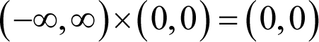
and hence
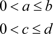
we define
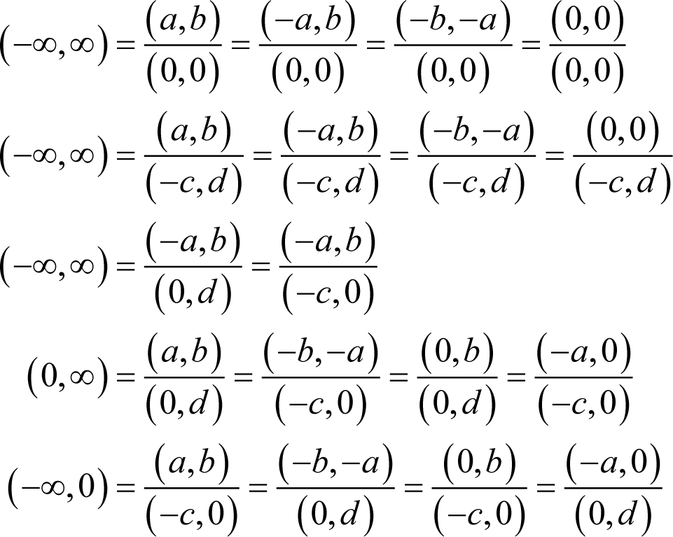
and
An interval class
Listing 1 gives the definition of an interval number class.
class interval
{
public:
  static void add_error(double &lb, double &ub);

  interval();
  interval(const double x);
  interval(const double lb, const double ub);

  double     lower_bound() const;
  double     upper_bound() const;
  bool       is_nan() const;
  int        compare(const interval &x) const;
  interval & negate();

  interval & operator+=(const interval &x);
  interval & operator-=(const interval &x);
  interval & operator*=(const interval &x);
  interval & operator/=(const interval &x);

private:
  double lb_;
  double ub_;
};
|
| Listing 1 |
In the constructors we shall assume that a value is inexact, unless the user explicitly passes equal upper and lower bounds or it is default constructed as 0. Note that the user can also capture measurement uncertainty with the upper and lower bound constructor.
The add_error static member function is provided to perform the error accumulation for both member and free functions. Its definition is provided in listing 2.
void
interval::add_error(double &lb, double &ub)
{
  static const double i
     = std::numeric_limits<double>::infinity();
  static const double e
     = std::numeric_limits<double>::epsilon();
  static const double m
     = std::numeric_limits<double>::min();
  static const double l = 1.0-e;
  static const double u = 1.0+e;

  if(lb==lb && ub==ub && (lb!=ub
     || (lb!=i && lb!=-i)))
  {
    if(lb>ub)  std::swap(lb, ub);

    if(lb>m)        lb *= l;
    else if(lb<-m)  lb *= u;
    else            lb -= e*m;

    if(ub>m)        ub *= u;
    else if(ub<-m)  ub *= l;
    else            ub += e*m;
  }
  else
  {
    lb = std::numeric_limits<double>::quiet_NaN();
    ub = std::numeric_limits<double>::quiet_NaN();
  }
}
|
| Listing 2 |
For the upper bound, this worst case will occur if we multiply by u when it is positive and by l when it is negative. This is because, for negative numbers, the greater numbers are those with smaller magnitudes. By the same argument the opposite is true for the lower bound.
Additionally we must take care to accumulate errors in denormal numbers additively.
Finally we exploit the fact that all comparisons involving NaNs are false to ensure that if either bound is NaN, both will be.
The implementations of the constructors, together with the trivial upper and lower bound data access methods are provided in listing 3.
interval::interval()
: lb_(0.0), ub_(0.0)
{
}

interval::interval(const double x)
: lb_(x), ub_(x)
{
  add_error(lb_, ub_);
}

interval::interval(const double lb,
                   const double ub)
: lb_(lb), ub_(ub)
{
  static const double i
     = std::numeric_limits<double>::infinity();

  if(lb==lb && ub==ub && (lb!=ub ||
     (lb!=i && lb!=-i)))
  {
    if(lb_>ub_)  std::swap(lb_, ub_);
  }
  else
  {
    lb_
       = std::numeric_limits<double>::quiet_NaN();
    ub_
       = std::numeric_limits<double>::quiet_NaN();
  }
}

double
interval::lower_bound() const
{
  return lb_;
}

double
interval::upper_bound() const
{
  return ub_;
}
|
| Listing 3 |
Negating an interval can be done without introducing any further error since it simply requires flipping the sign bit. Its implementation therefore simply swaps the upper and lower bound after negating them, as shown in listing 4.
{
  lb_ = -lb_;
  ub_ = -ub_;
  std::swap(lb_, ub_);
  return *this;
}
|
| Listing 4 |
Comparing intervals is a little more difficult. It’s clear enough what we should do if the two intervals don’t overlap, but it’s a little confusing as to what we should do if they do.
We could take the position that two intervals shall compare as equal if it is at all possible that they are equal. Unfortunately, this means that equality would no longer be transitive. An interval x might overlap y and y might overlap z despite x not overlapping z. We would therefore have to be extremely careful when dealing with equality comparisons. A simpler alternative that maintains transitivity of equality is to compare the midpoints of the intervals.
We shall use the second approach and its implementation is given in listing 5. Note that we must also provide an is_nan method to allow the comparison operators to behave correctly in their presence.
bool
interval::is_nan() const
{
  return !(lb_==lb_);
}

int
interval::compare(const interval &x) const
{
  const double lhs =   lb_*0.5 +   ub_*0.5;
  const double rhs = x.lb_*0.5 + x.ub_*0.5;

  if(lhs<rhs) return -1;
  if(lhs>rhs) return  1;
  return 0;
}
|
| Listing 5 |
When adding intervals we add their upper and lower bounds and then add further errors to the bounds, as shown in listing 6.
interval &
interval::operator+=(const interval &x)
{
  lb_ += x.lb_;
  ub_ += x.ub_;

  add_error(lb_, ub_);

  return *this;
}
|
| Listing 6 |
Subtracting intervals is similarly straightforward, as shown in listing 7.
interval &
interval::operator-=(const interval &x)
{
  lb_ -= x.ub_;
  ub_ -= x.lb_;

  add_error(lb_, ub_);

  return *this;
}
|
| Listing 7 |
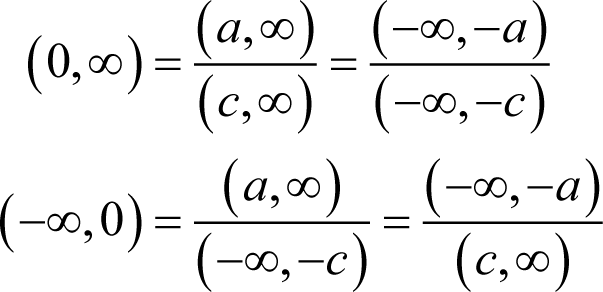
When multiplying intervals we must consider the effects of mixed positive and negative bounds. Specifically, we have 9 cases to consider
where each x and y value is greater than or equal to zero.
Rather than consider each case individually, I propose that we simply calculate all 4 products and pick out the least and the greatest. We can find the least of them reasonably efficiently with the first pass of a crude sorting algorithm. To find the greatest we can assign, rather than swap, values since we shan’t subsequently need the in-between values.
Note that if either argument is NaN we simply set the result to NaN. Having tested for this case, the only situation in which we shall come across NaNs is if we multiply an infinite bound by a zero bound, in which case we replace it with zero to reflect the fact that infinite bounds are open.
Listing 8 provides an implementation of multiplication.
interval &
interval::operator*=(const interval &x)
{
  if(!is_nan() && !x.is_nan())
  {
    double ll = lb_*x.lb_;
    double lu = lb_*x.ub_;
    double ul = ub_*x.lb_;
    double uu = ub_*x.ub_;

    if(!(ll==ll))  ll = 0.0;
    if(!(lu==lu))  lu = 0.0;
    if(!(ul==ul))  ul = 0.0;
    if(!(uu==uu))  uu = 0.0;

    if(lu<ll)  std::swap(lu, ll);
    if(ul<ll)  std::swap(ul, ll);
    if(uu<ll)  std::swap(uu, ll);

    if(lu>uu)  uu = lu;
    if(ul>uu)  uu = ul;

    lb_ = ll;
    ub_ = uu;

    add_error(lb_, ub_);
  }
  else
  {
    lb_
       = std::numeric_limits<double>::quiet_NaN();
    ub_
       = std::numeric_limits<double>::quiet_NaN();
  }

  return *this;
}
|
| Listing 8 |
When dividing, we must ensure that we properly handle denominators including zeros and infinities. Note that, similarly to how we did for multiplication, we exploit the fact that a NaN result from non NaN arguments identifies that both were infinities. We further exploit the fact that the lower bounds cannot be plus infinity nor the upper bounds minus infinity to replace such NaNs with the correct infinite bounds.
The cases of division by zero are handled by explicit branches and, as we did for multiplication, we find the lower and upper finite bounds with our crude sorting algorithm as shown in listing 9.
interval &
interval::operator/=(const interval &x)
{
  static const double i
     = std::numeric_limits<double>::infinity();
  if(x.lb_>0.0 || x.ub_<0.0)
  {
    double ll = lb_/x.lb_;
    double lu = lb_/x.ub_;
    double ul = ub_/x.lb_;
    double uu = ub_/x.ub_;

    if(!(ll==ll))  ll = i;
    if(!(lu==lu))  lu = -i;
    if(!(ul==ul))  ul = -i;
    if(!(uu==uu))  uu = i;

    if(lu<ll)  std::swap(lu, ll);
    if(ul<ll)  std::swap(ul, ll);
    if(uu<ll)  std::swap(uu, ll);

    if(lu>uu)  uu = lu;
    if(ul>uu)  uu = ul;

    lb_ = ll;
    ub_ = uu;

    add_error(lb_, ub_);
  }
  else if((x.lb_ <  0.0 && x.ub_ >  0.0)
       || (x.lb_ == 0.0 && x.ub_ == 0.0)
       || (  lb_ <  0.0 &&   ub_ >  0.0))
  {
    lb_ = -i;
    ub_ = i;
  }
  else if((x.lb_ == 0.0 && lb_ >= 0.0)
       || (x.ub_ == 0.0 && ub_ <= 0.0))
  {
    lb_ =  0.0;
    ub_ = i;
  }
  else if((x.lb_ == 0.0 && ub_ <= 0.0)
       || (x.ub_ == 0.0 && lb_ >= 0.0))
  {
    lb_ = -i;
    ub_ =  0.0;
  }
  else
  {
    lb_
       = std::numeric_limits<double>::quiet_NaN();
    ub_
       = std::numeric_limits<double>::quiet_NaN();
  }
  return *this;
}
|
| Listing 9 |
Aliasing
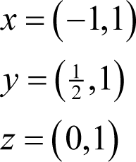
Unfortunately interval arithmetic is not entirely foolproof. One problem is that it can yield overly pessimistic results if an interval appears more than once in an expression. For example, consider the result of multiplying the interval (-1, 1) by itself.
Ignoring rounding error, doing so yields

rather than the correct result of (0,1).
This can be particularly troublesome if such expressions appear as the denominator in a division. For example, given
and again ignoring rounding errors, we have
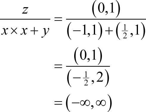
rather than
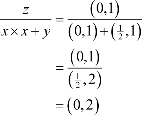
If we wish to ensure that such expressions yield as accurate results as possible we shall have to rearrange them so that we avoid aliasing. For example, rather than
x*x + 3.0*x - 1.0
we should prefer
pow(x+1.5, 2.0) - 3.25
Provided we keep in mind the fact that interval arithmetic can be pessimistic we can still use it naïvely to give us a warning of possible precision loss during a calculation.
Unfortunately there is a much bigger problem that we must consider.
Precisely wrong
Consider the use of our interval type in the calculation of the derivative of the exponential function at 1. The listing snippet below illustrates how we might calculate it for some leading number of zeros in δ, i.
  const interval d(pow(2.0, -double(i)));
  const interval x(1.0);
  const interval df_dx = (exp(x+d) - exp(x)) / d;
Note that since both x and δ are powers of 2, this code is needlessly pessimistic; they and their sum have exact floating point representations.
A more accurate approach is:
  const double d = pow(2.0, -double(i));

  const interval  x(1.0,   1.0);
  const interval xd(1.0+d, 1.0+d);

  const interval df = exp(xd) - exp(x);
  const interval df_dx(df.lower_bound()/d,
                       df.upper_bound()/d);
Note that in the final line we are also exploiting the fact that a division by a negative power of 2 is also exact when using IEEE floating point arithmetic.
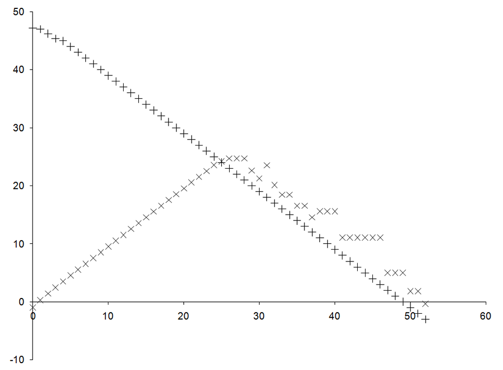
Figure 1 reproduces the graph of the error in the numerical approximation of the derivative together with the precision of that approximation. Specifically, it plots minus the base 2 logarithm of the absolute difference in the approximate and exact differentials, roughly equal to the number of correct bits, against minus the base 2 logarithm of δ, roughly equal to the number of leading zeros in its binary representation. On top of this it plots minus the base 2 logarithm of the difference between the upper and lower bounds of the approximate derivative, which is a reasonable proxy for the number of bits of precision in the result.
 |
| Figure 1 |
Clearly, there’s a linear relationship between the number of leading zeros and the lack of precision in the numerical derivate. Unfortunately, it is initially in the opposite sense to that between the number of leading zeros and the accuracy of the approximation.
We must therefore be extremely careful to distinguish between these two types of error. If we consider precision alone we are liable to very precisely calculate the wrong number.
So, whilst intervals are an extremely useful tool for ensuring that errors in precision do not grow to significantly impact the accuracy of a calculation, they cannot be used blindly. As has consistently been the case, we shall have to think carefully about our calculations if we wish to have confidence in their results.
I shall deem this type a roast duck; tasty, but quite incapable of flight.
Mmmm, quaaack.
You’re going to have to think!
We have seen that there are many ways in which we might represent numbers with computers and that they all convey certain strengths and weaknesses.
We have found that none of them can, in general, remove the need to think carefully about how we perform our calculations. For certain mathematical calculations, the algorithms we use to compute them and the implementation of those algorithms are by far the most important factors in keeping errors under control.
In consequence, I contend that double precision floating point arithmetic, being an efficient and parsimonious means to represent a vast range of numbers, is almost always the correct choice for general purpose arithmetic and that we must simply learn to live with the fact that we’re going to have to think!
Further reading
[Boost] http://www.boost.org/doc/libs/1_43_0/libs/numeric/interval/doc/interval.htm