Now we know our problem in depth. Richard Harris analyses if a common technique will work adequately.
In the previous article we discussed the foundations of the differential calculus. Initially defined in the 17 th century in terms of the rather vaguely defined infinitesimals, it was not until the 19 th century that Cauchy gave it a rigorous definition with his formalisation of the concept of a limit. Fortunately for us, the infinitesimals were given a solid footing in the 20 th century with Conway’s surreal numbers and Robinson’s non-standard numbers, saving us from the annoyingly complex reasoning that Cauchy’s approach requires.
Finally, we discussed the mathematical power tool of numerical computing; Taylor’s theorem. This states that for any sufficiently differentiable function f

If we do not place a limit on the number of terms, we have

Note that here f' ( x ) stands for the first derivative of f at x , f" ( x ) for the second and f ( n ) ( x ) for the n th with the convention that the 0 th derivative of a function is the function itself. The capital sigma stands for the sum of the expression to its right for every unique value of i that satisfies the inequality beneath it and i ! stands for the factorial of i , being the product of every integer between 1 and i , with convention that the factorial of 0 is 1.
You may recall that we used forward finite differencing as an example of cancellation error in the first article of this series [ Harris10 ]. This technique replaces the infinitesimal δ in the definition of the derivative with a finite, but small, quantity.
We found that the optimal choice of this finite δ was driven by a trade off between approximation error and cancellation error. With some fairly vigorous hand waving, we concluded that it was the square root of ε ; the difference between 1 and the smallest floating point number greater than 1.
This time, and I fancy I can hear your collective groans of dismay, we shall dispense with the hand waving.
Forward finite difference
Given some small finite positive δ , the forward finite difference is given by

Using Taylor’s theorem the difference between this value and the derivative is equal to

for some y between x and x + δ .
Assuming f introduces a relative rounding error of some non-negative integer n f multiples of ½ ε and that x has already accumulated a relative rounding error of some non-negative integer n x multiples of ½ ε then, if we wish to approximate the derivative as accurately as possible we should choose δ to minimise

as shown in derivation 1.
|
Approximation error of the forward finite difference From Taylor’s theorem we have
for some y between x and x + δ . We shall assume that f introduces a proportional rounding error of some non-negative integer n f multiples of ½ ε and that x has a proportional rounding error of some non-negative n x multiples of ½ ε . We shall further assume that we can represent δ exactly and that the sum of it and x introduces no further rounding error. Under these assumptions the floating point result of the forward finite difference calculation is bounded by
where the error in x is the same in both cases. This is in turn bounded by
Noting that
the result is hence bounded by
giving a worst-case absolute error of
|
| Derivation 1 |


Now this is a function of δ of the form

Such functions, for positive
a
,
b
and
x
, have a minimum value of
 at
at
 (taking the positive square roots) as shown in derivation 2.
|
The minimum of a / x + bx + c Recall that the turning points of a function f , that is to say the minima, maxima and inflections, occur where the derivative is zero.
Note that this is only a real number if a and b have the same sign. We can use the second derivative to find out what kind of turning point this is; positive implies a minimum, negative a maximum and zero an inflection.
If both a and b are positive and we choose the positive square root of their ratio then this value is positive and we have a minimum. |
| Derivation 2 |


To leading order in ε and δ the worst case absolute error in the forward finite difference approximation to the derivative is therefore

when δ is equal to

taking the positive square roots in both expressions.
Now these expressions provide a very accurate estimate of the optimal choice of δ and the potential error in the approximation of the derivative that results from that choice. There are, however, a few teensy-weensy little problems.
The first is that these expressions depend on the relative rounding errors of x and f . We can dismiss these problems out of hand since if we have no inkling as to how accurate x or f are then we clearly cannot possibly have any expectation whatsoever that we can accurately approximate the derivative.
The second, and slightly more worrying, is that the error depends upon the very value we are trying to approximate; the derivative of f at x . Fortunately, we can recover the error to leading order in ε by replacing it with the finite difference itself.
The third, and by far the most significant, is that both expressions depend upon the behaviour of the unknown second derivative of f .
Unfortunately this is ever so slightly more difficult to weasel our way out of. By which I of course mean that in general it is entirely impossible to do so.
Given the circumstances, the best thing we can really do is to guess how the second derivative behaves. For purely pragmatic reasons we might assume that

since this yields

The advantage of having a δ of this form is that it helps alleviate both rounding and cancellation errors; it is everywhere larger than (2 n f ε ) ½ | x | and hence mitigates against rounding error for large | x | and it is nowhere smaller than (2 n f ε ) ½ and hence mitigates against cancellation error for small | x |.
Substituting this into our error expression yields

Of course this estimate will be inaccurate if the second derivative differs significantly from our guess.
This is little more than an irritation if our guess is significantly larger than the second derivative since the true error will be smaller than our estimate and we will still have a valid, if pessimistic, bound.
If our guess is significantly smaller, however, we’re in trouble since we shall in this case underestimate the error. Unfortunately there is little we can do about it.
One thing worth noting is that if the second derivative is very large at x then the derivative will be rapidly changing in its vicinity. The limiting case as the second derivative grows in magnitude is a discontinuity at which the derivative doesn’t exist.
If we have a very large second derivative, we can argue that the derivative is in some sense approaching non-existence and that we should need to be aware of this and plan our calculations accordingly.
We have one final issue to address before implementing our algorithm; we have assumed that we can exactly represent both δ and x + δ . Given that our expression for the optimal choice of δ involves a floating point square root operation this is, in general, unlikely to be the case.
Fortunately we can easily find the closest floating point value to δ for which our assumptions hold with

Naturally this will have some effect on the error bounds, but since it will only be O ( εδ ) it will not impact our approximation of them.
Listing 1 provides the definition of a forward finite difference function object.
template<class F>
class forward_difference
{
public:
  typedef F function_type;
  typedef typename F::argument_type argument_type;
  typedef typename F::result_type result_type;

  explicit forward_difference(
     const function_type &f);
  forward_difference(const function_type &f,
                     unsigned long nf);

  result_type operator()(
     const argument_type &x) const;

private:
  function_type f_;
  result_type   ef_;
};
|
| Listing 1 |
Note that we have two constructors; one with an argument to represent n f and one without. The latter assumes a rounding error of a single ½ ε , as shown in listing 2, and is intended for built in functions for which such an assumption is reasonable.
template<class F>
forward_difference<F>::forward_difference(
  const function_type &f) : f_(f),
  ef_(sqrt(result_type(2UL)*eps<result_type>()))
{
  if(ef_<result_type(eps<argument_type>()))
  {
    ef_ = result_type(eps<argument_type>());
  }
}

template<class F>
forward_difference<F>::forward_difference(
  const function_type &f,
  const unsigned long nf) : f_(f),
  ef_(
     sqrt(result_type(2UL*nf)*eps<result_type>()))
{
  if(ef_<result_type(eps<argument_type>()))
  {
    ef_ = result_type(eps<argument_type>());
  }
}
|
| Listing 2 |
Note also that we are assuming that the result type of the function object has a
numeric_limits
specialisation (whose
epsilon
function is represented here by the typesetter-friendly abbreviation
eps
<T>
), can be conversion constructed from an unsigned long and has a global namespace overload for the
sqrt
function. To all intents and purposes we are assuming it is an inbuilt floating point type.
We should rather hope that the argument type of the function object is the same as its result type, and for that matter that this is a floating point type, but must provide for a minimum
δ
just in case the user decides otherwise, which we do by setting a lower bound for
ef_
. We must be content in such cases with the fact that they have made a rod for their own back when it comes time to perform their error analysis!
Listing 3 gives the implementation of the function call operator based upon the results of our analysis.
template<class F>
typename forward_difference<F>::result_type
forward_difference<F>::operator()(
   const argument_type &x) const
{
  const argument_type abs_x =
     (x>argument_type(0UL)) ? x : -x;
  const argument_type d =
     ef_*(abs_x+argument_type(1UL));
  const argument_type u = x+d;

  return (f_(u)-f_(x))/result_type(u-x);
}
|
| Listing 3 |
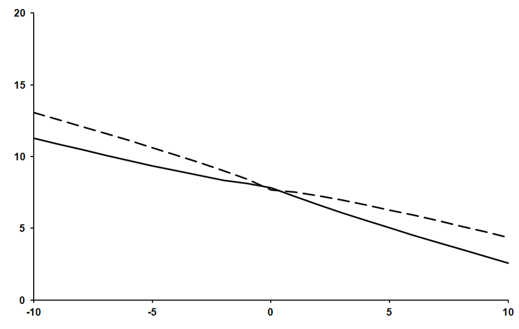
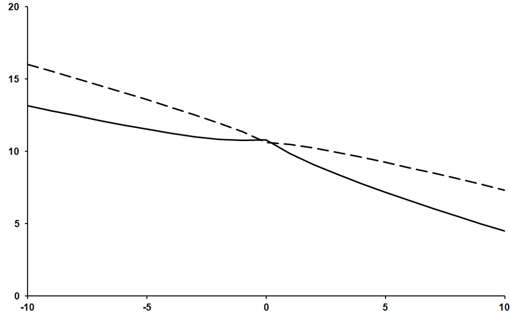
As an example, let us apply our forward difference to the exponential function with arguments from -10 to 10. We can therefore expect that n f is equal to one and n x to zero and hence that our approximation of the error is

Since the derivative of the exponential function is the exponential function itself, we can accurately calculate the true error by taking the absolute difference between it and the finite difference approximation.
To compare our approximation of the error with the exact error we shall count the number of leading zeros after the decimal point of each, which we can do by negating the base 10 logarithm of the values.
Figure 1 plots the leading zeros in the decimal fraction of our approximate error as a dashed line and in that of the true error as a solid line, with larger values on the y axis thus implying smaller values for the errors.
|
| Figure 1 |
Our approximation clearly increasingly underestimates the error as the absolute value of x increases. This shouldn’t come as too much of a surprise since our assumption about the behaviour of the second derivative grows increasingly inaccurate as the magnitude of x increases for the exponential function.
Nevertheless, our approximation displays the correct overall trend and is nowhere catastrophically inaccurate, at least to my eye.
The question remains as to whether we can do any better.
Symmetric finite difference
Returning to Taylor’s theorem we can see that the term whose coefficient is a multiple of the second derivative is that of δ 2 . This has the very useful property that it takes the same value for both + δ and - δ .
If we approximate the derivative with the finite difference between a small step above and a small step below x we can arrange for this term to cancel out. Specifically, the expression

differs from the derivative at x by

for some y between x - δ and x + δ as shown in derivation 3.
|
The symmetric finite difference From Taylor’s theorem we have
for some y 0 between x - δ and x and y 1 between x and x + δ The symmetric finite difference is therefore.
The intermediate value theorem states that for a continuous function, there must be a point x between points x 0 and x 1 such that
If the second derivative of our function is continuous this means that
for some y between x - δ and x + δ |
| Derivation 3 |


Now this is a rather impressive order of magnitude better in δ than the forward finite difference considering that it involves no additional evaluations of f .
That said, it is not at all uncommon that both the value of the function and its derivative are required, in which case the finite forward difference can get one of its function evaluations for free.
With a similar analysis to that we made for the forward finite difference, given in derivation 4, we find that the optimal choice of δ must minimise

|
Approximation error of the symmetric finite difference From Taylor’s theorem we have
for some y between x and x + δ . Making the same assumptions as before about rounding errors in both f and x , the floating point result of the symmetric finite difference calculation is bounded by
which is in turn bounded by
The error in x is again the same in all cases giving us
and hence a worst case absolute error of
or, by the mean value theorem again
|
| Derivation 4 |


This time the quantity we wish to minimise is a function in δ of the form

which, as shown in derivation 5, given positive b is minimised by

|
The minimum of a / x + bx 2 +c We find a turning point of f with
We have a second derivative of
so if b is positive we have a minimum. |
| Derivation 5 |


To leading order in ε and δ the minimum relative error in the symmetric finite difference approximation to the derivative is therefore

when δ is equal to

Now this error is
 and we should therefore expect this to be significantly better than the forward finite difference with its
 error.
Unfortunately in order to achieve this we have compounded the problem of unknown quantities in the error and the choice of δ .
The optimal choice of the δ is now dependent on the properties of the third rather than the second derivative of f so we cannot use our previous argument that it may in some sense be reasonable to ignore it.
Furthermore, the resulting approximation error is dependant on both the second and the third derivatives of f .
We can deal with the first problem in the same way as we did before. In the name of pragmatism we assume that

giving a δ of

It’s a little more difficult to justify a guess about the form of the second derivative since it plays no part in the choice of δ .
We could arbitrarily decide that it has a similar form to that we chose for it during our analysis of the forward finite difference. Specifically

This strikes me a vaguely unsatisfying however, since it is not consistent with our assumed behaviour of the third derivative.
Instead, I should prefer something that satisfies

since this is approximately consistent with our guess.
|
A consistent second derivative Consider first
where a is a constant and sgn( x ) is the sign of x . For simplicity’s sake, we shall declare the derivative of the absolute value of x at 0 to be 0 rather than undefined. The second term has the required form so if we can find a way to cancel out the first we shall have succeeded. Adding a second term whose derivative includes a term of the same form might just do the trick.
We therefore require
Solving for a and b yields a serendipitously unique result. |
| Derivation 6 |

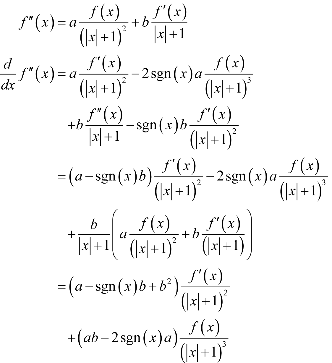
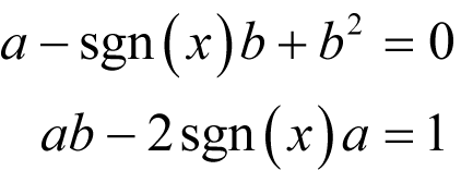
Derivation 6 shows that we should choose

for positive x ,

for x equal to zero and

for negative x , with terms given to 5 decimal places.
Substituting these guessed derivatives back into our error formula yields an estimated error of

for positive x ,

for x equal to zero and

for negative x .
Once again we shall not use δ directly, but shall instead use the difference between the floating point representations of x + δ and x - δ .
Listing 4 provides the definition of a symmetric finite difference function object.
template<class F>
class symmetric_difference
{
public:
  typedef F function_type;
  typedef typename F::argument_type argument_type;
  typedef typename F::result_type result_type;

  explicit symmetric_difference(
     const function_type &f);
  symmetric_difference(const function_type &f,
                       unsigned long nf);

  result_type operator()
     (const argument_type &x) const;

private:
  function_type f_;
  result_type   ef_;
};
|
| Listing 4 |
We again have two constructors; one for built in functions and one for user defined function, as shown in listing 5. Listing 6 gives the definition of the function call operator based upon our analysis.
template<class F>
symmetric_difference<F>::symmetric_difference(
  const function_type &f) : f_(f),
  ef_(pow(result_type(3UL)/result_type(2UL) *
      eps<result_type>(),
          result_type(1UL)/result_type(3UL)))
{
  if(ef_<result_type(eps<argument_type>()))
  {
    ef_ = result_type(eps<argument_type>())
  }
}

template<class F>
symmetric_difference<F>::symmetric_difference(
  const function_type &f,
  const unsigned long nf) : f_(f),
  ef_(pow(result_type(3UL*nf)/result_type(2UL) *
      eps<result_type>(),
          result_type(1UL)/result_type(3UL)))
{
  if(ef_<eps<argument_type>())
  {
    ef_ = eps<argument_type>();
  }
}
|
| Listing 5 |
template<class F>
typename symmetric_difference<F>::result_type
symmetric_difference<F>::operator()(
   const argument_type &x) const
{
  const argument_type abs_x =
     (x>argument_type(0UL)) ? x : -x;
  const argument_type d =
     ef_*(abs_x+argument_type(1UL));
  const argument_type l = x-d;
  const argument_type u = x+d;

  return (f_(u)-f_(l))/result_type(u-l);
}
|
| Listing 6 |
Figure 2 plots the negation of the base 10 logarithm of our approximation of the error in this numerical approximation of the derivative of the exponential function as a dashed line and the true error as a solid line.
|
| Figure 2 |
Clearly the error in the symmetric finite difference is smaller than that in the forward finite difference, although it appears that the accuracy of our approximation of that error isn’t quite so good. That said, the average ratios between the number of decimal places in the true error and the approximate error of the two algorithms are not so very different; 1.21 for the forward finite difference and 1.24 for the symmetric finite difference.
Still, not too shabby if you ask me.
But the question still remains as to whether we can do any better.
Higher order finite differences
As it happens we can, although I doubt that this comes as much of a surprise. We do so by recognising that the advantage of the symmetric finite difference stems from the fact that terms dependant upon the second derivative largely cancel out. If we can arrange for higher derivatives to cancel out we should be able to improve accuracy still further.
Unfortunately, doing so makes a full error analysis even more tedious than those we have already suffered through. I therefore propose, and I suspect that this will be to your very great relief, that we revert to our original hand-waving analysis.
In doing so our choice of δ shall not be significantly impacted, but we shall have to content ourselves with a less satisfactory estimate of the error in the approximation.
We shall start by returning to Taylor’s theorem again.

From this we find that the numerator of the symmetric finite difference is

Performing the same calculation with 2 δ yields

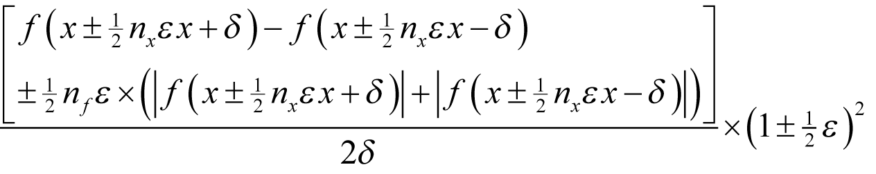
With a little algebra it is simple to show that

Assuming that each evaluation of
f
introduces a single rounding error and that the arguments are in all cases exact this mean that the optimal choice of
δ
is of order
 as shown in derivation 7.
|
The optimal choice of δ Noting that multiplying by a power of 2 never introduces a rounding error, the floating point approximation to our latest finite difference is bounded by
which simplifies to
The order of the error is consequently minimised when
|
| Derivation 7 |


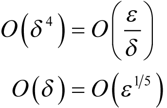
By the same argument from pragmatism that we have so far used we should therefore choose

to yield an
 error in our approximation.
With sufficient patience, we might continue in this manner, creating ever more accurate approximations at the expense of increased calls to f .
Unfortunately, not only is this extremely tiresome, but we cannot escape the fact that the error in such approximations shall always depend upon the behaviour of unknown higher order derivatives.
For these reasons I have no qualms in declaring finite difference algorithms to be a flock of lame ducks.
tutti: Quack!
Reference
[Harris10] Harris, R., ‘You’re Going to Have to Think; Why [Insert Technique Here] Won’t Cure Your Floating Point Blues’, Overload 99, ACCU, 2010