Diffusion models can be used in many areas. Frances Buontempo applies them to paper bag escapology.
Many applications in variety of areas from finance to epidemiology use Monte Carlo simulations of stochastic models, that is one using random variables. This article will revise the basics of Monte Carlo simulation and show how to simulate standard and geometric Brownian motion, ending with jump diffusion. The aim will simply be to move points out of a paper bag, since everyone should know how to program their way out of a paper bag. The simplest case, standard Brownian motion, simulates a cloud of particles spreading out, or diffusing, over time. This will allow us to introduce a mathematical model to simulate in code and form a basis for further simulations – geometric and jump diffusion. Both of these will show how a stock price might move over time. We will resort to cheating in order to make the price eventually end higher than the top of the bag. The reader can then decide if we have actually programmed our way out of a paper bag, or simply developed a simulation which allows discovery of appropriate parameters to meet a requirement. This, of course, is an essential use for much simulation software and will thereby demonstrate the value of coding up models to see what happens. The three diffusion models produce animations which move over time, so a paper article cannot do full justice to these. The code is available on github [ github ] for the reader to experiment with if desired.
Monte Carlo simulation
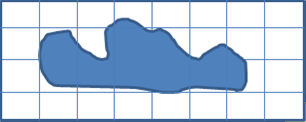
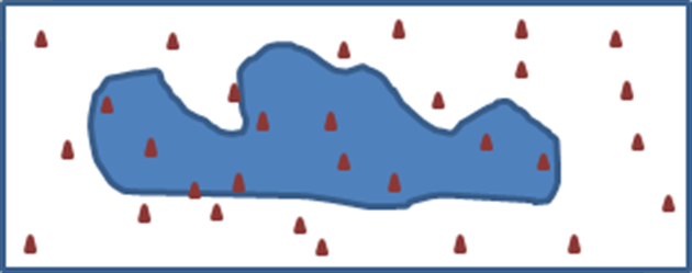
A Monte Carlo simulation allows one to answer, with varying degrees of accuracy, numerical problems that cannot be solved directly. For example, in order to find the area under a curve various approaches can be used. If the curve has a known equation which is integrable, the definite integral in the desired range can be calculated to give the area under part of the curve, or the indefinite integral will give the area under the whole curve. If the function describing the curve cannot be integrated, this approach will not work. If the curve were a hand drawn squiggle, we would not even have a function to attempt to integrate. In both cases, various estimation schemes may be used. Consider the curve in Figure 1. If a grid is superimposed, the area enclosed by the squiggle can be estimated by counting how many unit squares contain some of the interior of the curve. Finer grained grids will give more accurate estimates. Alternatively, a Monte Carlo simulation can be used, illustrated by the ‘darts’ in the last containing rectangle. If we randomly throw some darts, here 30, at the rectangle and find 10 are inside, we have 10/30 = 1/3 inside the curve, so around 33% of the area of the rectangle approximates the area inside the curve. Several such experiments will inevitably give varying areas, which may then be averaged or used to give a lower and upper bound as desired. The essence of any such simulation is the same; run an experiment a few times, and either see what happens, or try to answer a question. This introduction asked “What’s the area of a curve?” Our subsequent simulations will discover if we can diffuse our way out of a paper bag.

|
|
|
| Figure 1 |
Brownian motion
There are various diffusion equations as indicated in the introduction. Diffusion is a process whereby substances move, apparently randomly, from places of higher concentration to those with lower concentration, eventually reaching equilibrium. This can be at the molecular level, in solids, liquids and gases, driven by pressure, temperature or electrical energy. Further details are available in various resources, for example see [ Mostinsky ]. For our simplest case, Brownian motion describes the motion of particles bouncing around in a fluid – either a liquid or a gas. Since we wish to model particles escaping from a paper bag, it is prudent to use the gas model.
Brownian motion is a special case of a random walk. It is a Markov process; that is, it has no memory. At any moment in time, the next position depends on where it is now, not how it got there. Other types of random walks are non-Markovian, for example taking their steps at random times. Brownian motion has two further properties: it has a mean change of zero and its change has a variance equal to the time step. In fact, the change, or step, is normally distributed. These properties make it a Wiener Process [
Hull
]. To get an intuitive sense of this, consider a simple random walk with a step size of one along a line, either going left or right. After starting at an origin, 0, the first step will take a particle either left, -1, or right, +1, with equal probability. So, for several experiments of one step, we will have an average of 0 steps. For experiments of more steps, we still get an average of zero, since the average of the total number of steps, is the total of the average step. If we now consider the step sized squared, we get 1. The distance squared will always be more than zero. In fact, the average of the sum of squared steps will be the number of steps. This gives us the variance property. The details can be found elsewhere, but [
Schmidt
] gives a simple explanation. If we then allow the step size to vary, in particular following a Gaussian distribution with mean 0 and variance 1, we nearly have Brownian motion. If we do this for two dimensions we are there. Consider a particular at some point (x, y). Given a source of two independent Gaussian random variables, mean 0, variance 1, called φ
1
,φ
2
respectively, the particle will move to
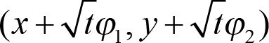 . To implement this, we can make two independent draws from one random number generator. We could let
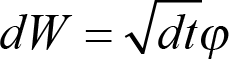 to simplify the equation.
Given a point, or particle starting at (x, y) we can then update it easily using a normal distribution in C++11 as seen in Listing 1. Details, such as the constructor implementation should be obvious, and how you would wish to report the current position is left to the reader. I used the Simple and Fast Media Library [ SFML ] to demonstrate the Brownian motion.
class Particle {

public:
  Particle(double root_t,
          double x = 0,
          double y = 0,
          unsigned int seed = 1);
  void Update() {
    x += move_step();
    y += move_step();
  }

private:
  double root_t;
  double x;
  double y;
  std::mt19937 engine;
  std::normal_distribution<T> normal_dist;
  double move_step() {
    return root_t * normal_dist(engine);
  }

};
|
| Listing 1 |
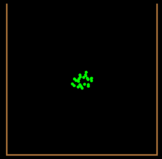
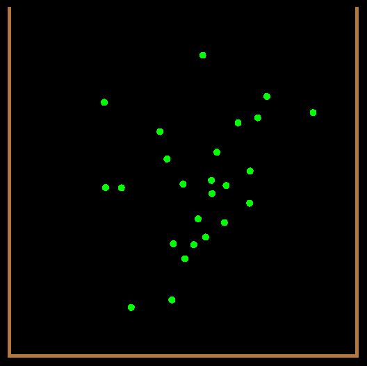
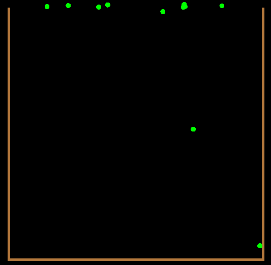
If we initialise several particles in the centre of a ‘paper bag’, indicated by three edges, and leave them to update according to this simple formula, they gradually diffuse. The greater the time step the faster they move. The next set of figures (Figure 2) does indeed show a cloud of particles spreading out from the centre. The more astute reader may have realised that since each direction is equally likely the particles are quite free to sneak back inside the bag, even if briefly. It is possible to add paper bag edge detection to stop this happening, though this slows the dispersion down. The final figure shows some particles stopped just above the bag, since the code makes them stop when they have escaped from a paper bag.
|
|
|
| Figure 2 |
Geometric Brownian motion
We have seen how simple the Brownian motion simulation was. Since this allows particles to move freely in two dimensions, they will either go through the sides of the paper bag, or if constrained not to, eventually go out of the top of the bag. If we now simulate a model of stock prices tending to go up, this will get us out of the bag more quickly. In order to do this we will use geometric Brownian motion. This is very similar to the first model. The logarithm of our new quantity follows Brownian motion but the process also has drift. In other words, taking the exponential of a Brownian motion with drift gives us geometric Brownian motion. This time, our quantity will be a fictitious stock price, S, giving us the y-coordinate, and we can just use the time, t, instead of an x-coordinate.
This stochastic differential equation can be discretised taking a previous stock price S and the step to the next stock price as ΔS = S(
μ
Δ
t
+
σ
Δ
W
). Adding this step to the previous price gives us the next price. We still have the
dW
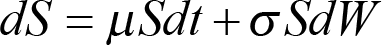
as before, but now we have a drift, μ, which is the rate of return on our investment, and a scale parameter, σ, which is usually described as volatility in a finance context. If this is zero, we have ‘turned off’ the stochastic, or random, part of the model and just see a simulation of the returns from a completely secure investment with a known return. Different stochastic differential equations (SDEs) will have different discretisation schemes, where we move from a stochastic differential equation to the move in a discrete step. Another common SDE is
 .
.
Given an initial stock price, and a drift and volatility parameter it is then easy to generate a sequence of possible stock prices after each time step, dt. This is shown in Listing 2.
class PriceSimulation {
public:
  PriceSimulation(double price, double drift,
                  double vol, double dt,
                  unsigned int seed);
  double update() {
    double stochastic = normal_dist(engine);
    double increment =
      drift * dt + vol * sqrt(dt) * stochastic;
    price += price * increment;
    return price;
  }

private:
  std::mt19937 engine;
  std::normal_distribution<> normal_dist;
  double price;
  double drift;
  double vol;
  double dt;
};
|
| Listing 2 |
If we treat the left most side of a paper bag, again indicated by three lines – a left side, the bottom and a right side, we can start the stock price somewhere above the bottom of the bag, which would be a value of 0, and see what happens. Clearly, if the stock is initially zero, each step ΔS will be zero since
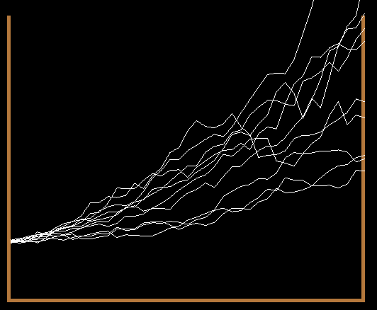
 . Any initial stock value greater than zero will do. Similarly, if we take the left most side of the bag as time 0, and simulate the potential stock prices over a couple of years, each result can be plotted with a line drawn between each sample point. These then give scales for displaying the results. Figure 3 shows what happens with 10 simulations, using time steps of 0.1, with a drift of 0.5 and volatility of 0.2.
|
| Figure 3 |
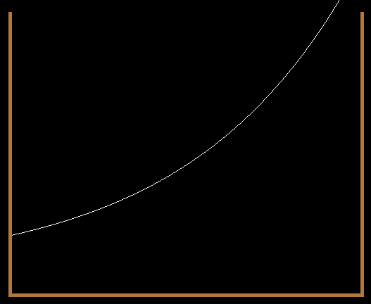
As expected the lines do resemble a stock price moving upwards over time. Unfortunately many of the final prices fail to end out of the bag. Some thought, or some time tweaking the parameters reveals that turning off the volatility and ramping up the drift to over 50% (recall this is a made up stock offering, sorry to disappoint!) will cause all of the simulated paths to escape the paper bag. This is shown in Figure 4. Since we have turned off the volatility, the stochastic variable will be zero, and each path of stock prices is deterministic and therefore follows the same path.
|
| Figure 4 |
Jump diffusion
Resorting to turning off the volatility in the previous diffusion model is disappointing. With a higher drift rate and smaller volatility it is possible to end with most of the simulation paths escaping the paper bag. An alternative is to introduce jumps into the simulation. A key point of the Brownian motion models is their continuity. This is a precise mathematical concept, but it is sufficient to say a line or path is continuous if it can be drawn without taking your pen off the paper. A discontinuous path will have a jump – a point where the path breaks and pick up elsewhere. Jump diffusion can be used for a variety of application areas, but was introduced by Merton for financial pricing [ Merton ] and is often used in credit risk models. Without going into too many details, our initial stock model only allows each stock price change to be relatively small. A jump diffusion model will allow occasional large jumps, which might be more realistic. If we cheat and force these jumps to be positive, we are more likely to escape the paper bag. The obviously probability distribution to use to simulate something happening occasionally is the Poisson distribution. Calling this dN gives a stock price move in time dt of ΔS = S( μ Δ t + σ Δ W + J Δ N ) where J is the jump size. When dN gives us 0, this collapses to our previous model. When it is non-zero we have introduced a discontinuity. It is not immediately obvious whether it is ok to use the same underlying generator for both dW and dN [ StackOverflow ] however, for this simple demonstration it suffices.
This requires a relatively small change to our
PriceSimulation
class. A new member variable is required :
std::poisson_distribution<> poisson_dist;
This is initialised with the probability of jumping, which can be passed through from the command line. The new update function is shown in Listing 3.
double PriceSimulation::update() {
  double stochastic = normal_dist(engine);
  double dn = poisson_dist(engine);
  double increment  =
               drift * dt
               + vol * sqrt(dt) * stochastic
               + jump * dn;
  price += price * increment;
  return price;
}
|
| Listing 3 |
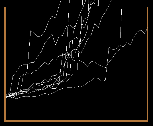
Figure 5 shows one outcome of our new jump diffusion model with 10 paths, time step 0.1, drift 0.5, volatility 0.2 and a jump size of 1 with a 50% chance of jumping. This time the majority of the stock price paths have managed to escape the paper bag. We could drop the drift and increase the probability of jumping in order to ensure the majority of paths escape. This indicates how useful coding up a model in order to experiment with the parameters can be.
|
| Figure 5 |
Conclusion
This article has given an overview Brownian motion, geometric Brownian motion and jump diffusion. We have not considered how many simulations would be required to give realistic models. The accuracy of such a simulation improves with the square root of the number of runs, so a vast number are often required. Other approaches can mitigate this, for example antithetic variates can be used as a variance reduction technique – if dW gives us stochastic variable w we form a second path at the same time using -w. Another approach is the use of so-called ‘low discrepancy numbers’ rather than pseudo-random numbers. Both methods are beyond the scope of this short article. Further details can be found in the literature, for example see [ Jäckel ].
This article aimed to show how useful Monte-Carlo simulations can be, and gave a high level description of some diffusion models. The reader is encouraged to try to program their own way out of a paper bag and is free to use the github code, or snippets herein as a starting point.
Acknowledgements
My heartfelt thanks to Cassio Neri for taking time to read through this article and stop me from using an incorrect discretization for an SDE. I hope this has made the article both easy to read, and equally importantly, correct.
References
[github] https://github.com/doctorlove/paperbag
[Hull] p265 John C. Hull Options, Futures and other Derivatives . 6th Edition
[Jäckel] 2002 Monte-Carlo methods in finance . Wiley.
[Merton] 1976, ‘Option pricing when underlying stock returns are discontinuous’. Journal of Financial Economics 3: 125-144
[Mostinsky] ‘Diffusion’ http://www.thermopedia.com/content/695/
[Schmidt] http://www.mit.edu/~kardar/teaching/projects/chemotaxis(AndreaSchmidt)/random.htm
[SFML] http://www.sfml-dev.org/
[StackOverflow] http://stackoverflow.com/questions/9870541/using-one-random-engine-for-multi-distributions-in-c11