Compilers are good at optimising modular calculations. Can we they do better? Cassio Neri shows they can.
Searching for ‘fast divisibility’ on Stack Overflow indicates that the question of whether hand-written C/C++ code can be faster than using the % operator fosters the curiosity of a few developers. Some answers basically state “Don’t do it. Trust your compiler.” I could not agree more with the principle. Compilers do a great job of optimising code and programmers should favour clarity. Nevertheless, this series shows ways to get improved performance when evaluating modular expressions. The intention here is not to ‘beat’ the compiler. On the contrary, this series is an open letter addressed to compiler writers presenting some algorithms that, potentially, could be incorporated into their product for the benefit of all programmers. Performance analysis shows that the alternatives discussed in this series are often faster than built-in implementations. With the exception of one algorithm which (to the best of my knowledge) is original, the others are not. Indeed, they have been covered by the classic Hacker’s Delight [ Warren ] for more than a couple of years. Nevertheless, major compilers still do not implemented them.
Warm up
We start looking at an example of the improvement that can be achieved. Figure 1 1 graphs the time it takes to check whether each element of an array of 65536 uniformly distributed unsigned 32-bits dividends in the interval [0, 1000000] leaves a remainder 3 when divided by 14.

|
| built_in<14> minverse<14> Noop |
|
ratio (CPU time / Noop time)
Lower is faster |
| Figure 1 |
This is performed by two in-line functions: the first one, labelled built_in , contains a single return statement:
return n % 14 == 3;
The one labelled minverse implements the modular inverse algorithm ( minverse for short) which is this article’s subject. Both measurements include the time to scan the array of dividends without performing any modular calculation. This time is also plotted against the label Noop and it is used as unit of time. The times 2 taken by minverse and the built-in algorithms are, respectively, 2.74 and 3.70. Adjusted times (obtained by subtracting the array scanning time) are then 2.74 - 1.00 = 1.74 and 3.70 - 1.00 = 2.70, which implies a ratio of 1.74 / 2.70 = 0.64. This represents a respectable 36% performance improvement with respect to the built-in algorithm. This ratio largely depends on the divisor, as will be made clear later on in this article.
Listings 1 and 2 contrast the code generated by GCC 8.2.1 (optimisation level at
-O3
) for the two algorithms. Although code size is not a perfect indication of speed, these two aspects are highly correlated.
built_in 0: 89 fa mov %edi,%edx 2: b9 93 24 49 92 mov $0x92492493,%ecx 7: d1 ea shr %edx 9: 89 d0 mov %edx,%eax b: f7 e1 mul %ecx d: c1 ea 02 shr $0x2,%edx 10: 6b d2 0e imul $0xe,%edx,%edx 13: 29 d7 sub %edx,%edi 15: 83 ff 03 cmp $0x3,%edi 18: 0f 94 c0 sete %al 1b: c3 retq |
| Listing 1 |
minverse 0: 83 ef 03 sub $0x3,%edi 3: 69 ff b7 6d db b6 imul $0xb6db6db7,%edi,%edi 9: d1 cf ror %edi b: 81 ff 92 24 49 12 cmp $0x12492492,%edi 11: 0f 96 c0 setbe %al 14: c3 retq |
| Listing 2 |
Preliminaries
This series of articles concerns the evaluation of modular expressions where the divisor is a compile time constant and the dividend is a runtime variable. Dividend and divisor have the same unsigned integer type.
The algorithms were implemented in a C++ library called qmodular [ qmodular ], short for quick modular . They can be implemented in standard C/C++ but qmodular uses a few GCC extensions including inline assembly. Our discussion focuses on GCC 8.2.1 for an x86_64 target but it is applicable to other compilers and architectures.
A fundamental reason for the currently built-in algorithm not being the most performant is that often it needlessly calculates remainders. For instance,
n % d == m % d
is, roughly speaking (more on this later), equivalent to
(n - m) % d == 0
. In this approach, there is no need to compute either
n % d
or
m % d
. However, the compiler evaluates both and ends up doing two modular calculations rather than one.
The built-in algorithm
For any given divisor, the compiler selects the best algorithm it knows for this particular value. Undoubtedly, the best case is where
d
is a power of two and
n % d
is evaluated as
n & (d – 1)
. This is a classic bitwise trick [
Warren
]. For other divisors,
n % d
is evaluated by the equivalent expression
n - (n / d) * d
. (Recall that
/
is integer division.) Hence,
n % d == r
becomes
n – (n / d) * d == r
.
The most important and widely implemented optimisation replaces the expensive division with a multiplication (instruction
mul
in Listing 1) by a ‘magic’ number (the constant
0x92492493
) and other cheap operations. Additional more trivial micro-optimisations are also applied. Two examples of such micro-optimisations follow.
When
r
is known to be zero at compile time, the subtraction is avoided and the expression is evaluated as
n == (n / d) * d
.
As mentioned earlier, when evaluating
n % d == m % d
, the compiler computes both remainders and, for each of them, performs a multiplication by the ‘magic’ number. Rather than twice loading this number into a register, this is done only once.
The modular inverse algorithm
This section covers the basics of the
minverse
algorithm by means of an example. A more detailed exhibition, including a mathematical proof of correctness, is provided in [
qmodular
]. We are interested in the case where
n
,
d
and
r
are unsigned integer numbers usually of 32 or 64 bits. For easy of exposition, we assume the number of bits is just 4 and hence,
n
ϵ Ω
4
= {0, …, 15}, which is a set small enough to allow manual inspection of all possible dividends. For this example we set the divisor
d
= 6.
Any strictly positive integer is a product of a positive odd number and a power of two. The algorithm starts by finding this decomposition for the divisor. In our example, d = 6 = 3∙2 1 and we set h = 3 and k = 1 (the exponent of 2). Since h is odd, by well known arithmetical results, there exists a unique g ϵ Ω 4 such that g ∙ h ≡ 1 (mod 2 4 ). Indeed, 11∙3 = 33 = 2∙2 4 + 1 and thus g = 11. More generally, the modulus can be any power of two, 2 w . (Again, the cases of practical interest are w = 32 and w = 64 but here we take w = 4.) Numbers g and h are said to be modular inverse (modulo 2 w ) of one another and hence the algorithm’s name.
For any n ϵ Ω w = {0, …, 2 w - 1}, let ror w ( n , k ) ϵ Ω w be obtained by rotating the bits of n by k positions to the right. For instance, ror 4 (3, 2) = 12 since 3 = (0011) 2 and 12 = (1100) 2 .
Given n ϵ Ω w , the algorithm proceeds with the calculation of ror w ( g ∙ n , k ). Table 1 shows detailed steps to get ror 4 (11∙ n , 1) for every n ϵ Ω 4 . (Rows are ordered by the last column.) One can easily inspect two crucial properties of the map n → ror w (g∙ n , k ): it is bijective and for multiples of d it matches division by d , that is, ror w ( g ∙ d ∙ i , k ) = i . (See first three rows.) This map has other interesting 3 properties but the two cited here are enough for the algorithm to work.
|
|||||||||||||||||||||||||||||||||||||||||||||||||||||||||||||||||||||||||||||||||||||
| Table 1 |
Let N r be the number of elements of Ω w that are equivalent to r (mod d ) and n = d ∙ i + r , with 0 ≤ i < N r , be one of them. Then n - r = i ∙ d and we obtain ror w ( g ∙( n - r ), k ) = i < N r . Reciprocally, if n ϵ Ω w is not equivalent to r (mod d ), then n - r is not multiple of d and ror w ( g ∙( n - r ), k ) ≥ N r .
In our example d = 6. Take, for instance, r = 2 and note the numbers in Ω 4 that leave this remainder when divided by d = 6, namely, 2, 8 and 14. From this we get N r = 3. Subtracting r = 2 from these three numbers yields 0, 6 and 12, respectively. They are mapped by n → ror w ( g ∙ n , k ) into 0, 1 and 2, which are exactly the elements of Ω 4 smaller than N r = 3.
In summary, given d = h ∙2 k , with h odd and 0 ≤ r < d , we have n ≡ r (mod d ), if and only if ror w ( g ∙( n – r ), k ) < N r , where g is the modular inverse of h (mod 2 w ) and N r is the number of elements of {0, …, 2 w - 1} that are equivalent to r (mod d ). Notice that g and k depend on d only and can be computed at compile time. However, N r depends on d and r . It can be known at compile time provided that r is.
At this point, Listing 2 becomes much less cryptic as the code generated for
  unsigned k = 1, g = 0xb6db6db7, r = 3,
    N = 0x12492493;
  return ror(g * (n – r), k) <= N - 1;
The snippet above calls the function
ror
, defined in
qmodular
, which is translated to the assembly instruction with the same name.
As in the built-in case, micro-optimisations can be applied. For instance, when
r == 0
the subtraction from
n
can be elided. The same holds for the multiplication, when
g == 1
, and for
ror
, when
k == 0
. These optimisations are performed by the compiler and we should not worry about doing them ourselves. However, there is another trick that the compiler cannot figure out by itself. It is based on a property of our map that we have not yet used. To each divisor, there corresponds a special remainder s ≠ 0 for which the subtraction can be eliminated provided the comparison is reversed. More precisely,
n
≡
s
(mod
d
), if and only if
ror
w
(
g
∙
n
,
k
) ≥ 2
w
-
N
r
. For instance, in Table 1 we see the three numbers leaving remainder 1, namely, 1, 7 and 13 are mapped, respectively, into 13, 14 and 15. Hence, the remainder is 1, if and only if the result is greater than or equal to 13 = 16 - 3 = 2
w
-
N
r
.
For evaluation of
n % d == m % d
, we use the fact that
n
≡
m
(mod
d
), if and only if
n
-
m
≡ 0 (mod
d
). Because unsigned types implement modulo 2
w
arithmetic (not modulo
d
) extra care must be taken for the subtraction not to underflow. Hence, we apply the test to either
n
-
m
or
m
-
n
depending on whether
n
≥
m
or not, that is,
n % d == m % d
can be evaluated as follows:
ror(g * (n >= m ? n - m : m - n), k) < N;
In reality, digressing from the modular inverse algorithm, this last reasoning equally applies to the built-in algorithm:
(n >= m ? n - m : m - n) % d == 0;
This way, the compiler calculates just one remainder instead of two as we have mentioned earlier. For the sake of completeness, the performance analysis includes the expression above.
The unbounded case
An implicit assumption of the previous section is that remainders are bounded,
r
<
d
, otherwise the modular inverse algorithm does not work. Since this condition does not always hold,
qmodular
implements two functions similar to those in Listing 3. The first one is as in the previous section and assumes
r < d
. The second function tests the condition and delegates the call to the first one.
bool
modular_inverse_bounded(unsigned n, unsigned r)
{
  /* ... */
}

bool
modular_inverse_unbounded(unsigned n, unsigned r)
{
  return r < d & modular_inverse_bounded(n, r);
}
|
| Listing 3 |
When
r
is known at compile time the compiler can figure out by itself whether
r < d
or not. In the affirmative case, the test is removed altogether and the second function simply calls and returns the result of the first one. Similarly, the negative case is reduced to
return false
.
Some readers might be thinking the
&
(bitwise
and
) in Listing 3 is a typo and
&&
(logical
and
) was intended. In reality, this is intentional. Due to short circuiting,
&&
yields a branch and performance suffers accordingly. Since computations in
modular_inverse_bounded
are cheap, it is much more efficient to carry them out rather then aborting evaluation when the first condition is false.
Performance analysis
As in the warm up, all measurements shown in this section concern the evaluation of modular expressions for 65536 uniformly distributed unsigned 32-bits dividends in the interval [0, 1000000]. Remainders can be either fixed at compile time or variable at runtime. Charts show divisors are on the x-axis and time measurements, in nanoseconds, on the y-axis. Timings are adjusted to account for the time of array scanning.
For clarity we restrict divisors to [1, 50] which suffices to spot trends. (Results for divisors up to 1000 are available in [ qmodular ].) In addition, we filter out divisors that are powers of two since the bitwise trick is undoubtedly the best algorithm for them. The timings were obtained with the help of Google Benchmark [ Google ] running on an AMD Ryzen 7 1800X Eight-Core Processor @ 3600Mhz; caches: L1 Data 32K (x8), L1 Instruction 64K (x8), L2 Unified 512K (x8), L3 Unified 8192K (x2).
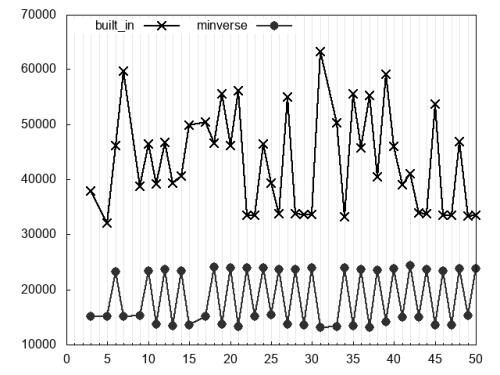
Figure 2 concerns the evaluation of
n % d == 0
and plots times taken by the built-in and
minverse
algorithms. The latter is clearly faster than the former.
Minverse
’s pretty regular zigzag is due to the microoptimisation that removes
ror
, if and only if
k
= 0. That is,
ror
is used for all even divisors and only for them.
|
| Figure 2 |
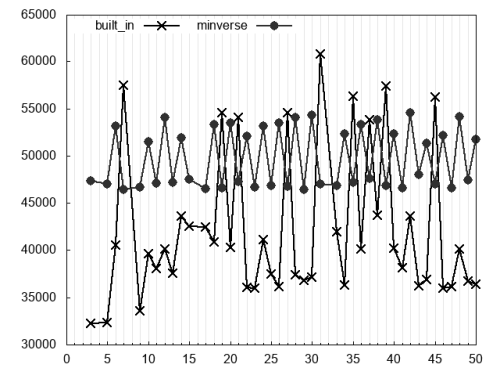
Figure 3 covers
n % d == r
where
r
is variable and uniformly distributed in [0,
d
). Despite the validity of precondition
r < d
, the compiler cannot know this and the boundness check is kept in the assembly code. Compared to the case of a fixed remainder, the built-in’s performance barely changes whereas
minverse
becomes visibly slower. This is due to the computation of
N
r
now being performed at runtime.
|
| Figure 3 |
For most divisors the built-in algorithm is faster than minverse . There are exceptions, though. Such divisors, up to 50, can be clearly seen in the chart and are 7, 19, 21, 27, 31, 35, 37, 39 and 45. The blame lies in the ‘magic’ number. For these divisors, corresponding ‘magic’ numbers do not fit in 32-bits registers. Consequently, they are truncated and more instructions are needed to correct the result. (I would like to point out to an interesting work [ ridiculous_fish ] which suggests alternative ways of dealing with such divisors. An idea very much worth exploring.)
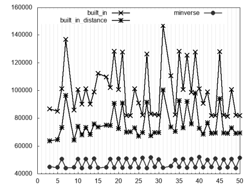
Finally, Figure 4 considers the expression
n % d == m % d
where both
n
and
m
are variable. As announced earlier, we also consider the variation that uses the absolute difference of
n
and
m
:
|
| Figure 4 |
(n >= m ? n – m : m – n) % d == 0;
This variation is labelled built_in_distance . Comparing this to the plain built-in algorithm we can see how effective this simple optimisation is. Nevertheless, minverse is still the fastest (it also uses the trick above).
Good and bad news regarding GCC 9.1
Starting at version 9.1, GCC implements the modular inverse algorithm. This welcome fact can be easily verified in [ godbolt ] by comparing the code generated for the following snippet with the code shown in Listing 2:
  bool f(unsigned n) {
    return n % 14 == 3;
  }
With GCC 8.2 for a x86-64 machine we obtain the code in Listing 4, and using GCC 9.1, we obtain the code in Listing 5.
movl %edi, %edx movl $-1840700269, %ecx shrl %edx movl %edx, %eax mull %ecx shrl $2, %edx imull $14, %edx, %edx subl %edx, %edi cmpl $3, %edi sete %al ret |
| Listing 4 |
imull $-1227133513, %edi, %edi subl $613566757, %edi rorl %edi cmpl $306783378, %edi setbe %al ret |
| Listing 5 |
A small difference between qmodular ’s implementation described here and GCC’s is worth mentioning because of its performance implications: while qmodular computes g ∙( n - r ), GCC computes g ∙ n - g ∙ r . It would be very costly to compute g ∙ r at runtime and, therefore, GCC only selects the minverse algorithm when the remainder is a compile time constant. (Even though and as we have seen, for some divisors minverse can beat the classic built-in algorithm.) Second, when r is a compile time constant it appears as an immediate value in the assembly code seen in Listing 2. In GCC’s implementation we see g ∙ r instead. Now, for (not so) small divisors and dividends (which is probably the most common case in practice), r is also small but g ∙ r is large. As it turns out, there are limitations on 64-bit immediate values which might force GCC’s implementation to use more instructions and registers.
Unfortunately, there seems to be yet another other issue with GCC’s implementation of
minverse
. For instance, for reasons unknown to me, changing the remainder from
3
to
4
is enough for the generated assembly to fall back to the old algorithm. Finally, regarding
n % d == m % d
, GCC does not use
minverse
at all and, instead, it computes the two remainders and compares them.
Conclusion
This article presents the modular inverse algorithm that can be used to evaluate expressions
n % d == r
and
n % d == m % d
. This algorithm is not new [
Warren
] but has not been widely implemented by compilers. Version 9.1 of GCC does implement it but there is room for further improvements. This work is intended to help compiler writers consider when they should use the modular inverse algorithm rather than what they currently use.
The greatest drawback regarding the
minverse
algorithm is that, to the best of my knowledge, it can not be efficiently used for other types of expressions like
n % d < r
or
n % d ≤ r
. These expressions and alternative algorithms for their evaluations are covered in Part II and Part III of this series.
Acknowledgements
I am deeply thankful to Fabio Fernandes for the incredible advice he provided during the research phase of this project. I am equally grateful to the Overload team for helping improve the manuscript.
References
[godbolt] https://godbolt.org/z/a7wr3U
[Google] https://github.com/google/benchmark
[qb] http://quick-bench.com/mhIaqB1ZvsBVROTGaO9opgx5ZTE
[qmodular] https://github.com/cassioneri/qmodular
[ridiculous_fish] ridiculous_fish, Labor of Division (Episode III): Faster Unsigned Division by Constants, October 19th, 2011, available at: http://ridiculousfish.com/blog/posts/labor-of-division-episode-iii.html
[Warren] Henry S. Warren, Jr., Hacker's Delight, Second Edition, Addison Wesley, 2013
- Powered by quick-bench.com [ qb ]. For readers who are C++ programmers and do not know this site, I strongly recommend to check it out. In addition, I politely ask all readers to consider contributing to the site to keep it running. (Disclaimer: apart from being a regular user and donor, I have no other affiliation with this site.)
-
YMMV, reported numbers were obtained by a single run in quick-bench.com using GCC 8.2 with
-O3and-std=c++17. - More generally, for any r (not necessarily zero), numbers leaving remainder r are strictly increasingly mapped into (disjoint) intervals. For instance, 1, 7 and 13 leave remainder 1 and are mapped to {13, 14, 15}, whereas 4 and 10 leave remainder 4 and are mapped into {6, 7}. Boundaries from shaded to unshaded rows mark remainder changes.
has a PhD in Applied Mathematics from Université de Paris Dauphine. He worked as a lecturer in Mathematics before moving to the financial industry.